Week 5 - Curve fitting

1. What does popt and pcov mean? (Watch the video to get some context)

" popt " is an array that stores the values of the coefficients that are being passed in a given function .

" pcov " is an two dimensional array that stores the values of the estimated covarience of popt i.e the coefficients .

2. What does np.array(temperature) do?

The above command is used for passing the vales of temperature as a numpy array .

3. What does the * in *popt mean?

" popt " is an array that stores the values of the coefficients that are being passed in a given function .

4. Write code to fit a linear and cubic polynomial for the Cp data. Explain if your results are good or bad.

Linear

import numpy as np
import matplotlib.pyplot as plt
from scipy.optimize import curve_fit 

def func(t,a,b):
       return a*t + b

def read_file():
	temp = []
	cp = []
	for line in open ('data','r'):        
	    values = line.split(',')           
	    temp .append(float(values[0]))    
	    cp.append(float(values[1]))

	return [temp,cp]   



temp,cp = read_file()                     
popt,pcov = curve_fit(func,temp,cp)       
fit_cp = func(np.array(temp), *popt)       


plt.plot(temp,cp,color="red",linewidth=3)
plt.plot(temp,fit_cp,color="green",linewidth=3)
plt.legend(['actual data','curve fit data'])
plt.xlabel('temperature [K]')
plt.ylabel('cp')
plt.savefig('Linear.png')
plt.show()

Output

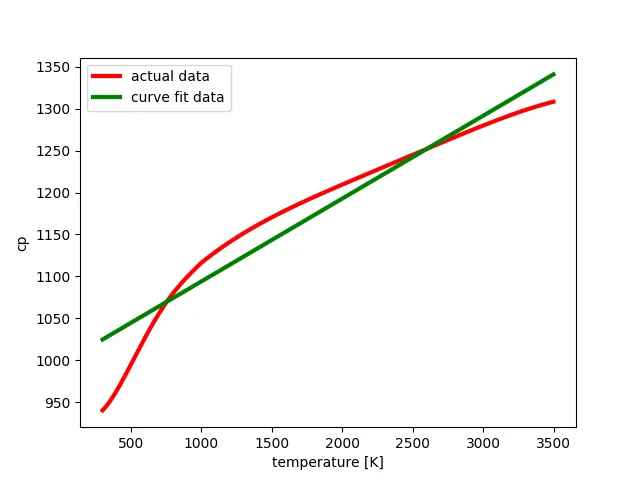
Explaining if the results are good or bad

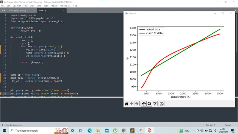
by using the linear curve to fit the given data, the plot is not so satisfying beacuse the original curve of the observed data looks like of quadratic or cubic nature. the linear curve has a lot of variation in comparision to the actual curve so the results are bad by using a linear equation.

Main Window

cubic polynomial

import numpy as np
import matplotlib.pyplot as plt
from scipy.optimize import curve_fit 

def func(t,a,b,c,d):
       return a*pow(t,3)+ b*pow(t,2) + c*t + d

def read_file():
	temp = []
	cp = []
	for line in open ('data','r'):        
	    values = line.split(',')          
	    temp .append(float(values[0]))    
	    cp.append(float(values[1]))

	return [temp,cp]   



temp,cp = read_file()
popt,pcov = curve_fit(func,temp,cp)      
fit_cp = func(np.array(temp), *popt)      


plt.plot(temp,cp,color="red",linewidth=3)
plt.plot(temp,fit_cp,color="green",linewidth=3)
plt.legend(['actual data','curve fit data'])
plt.xlabel('temperature [K]')
plt.ylabel('cp')
plt.savefig('Cubic Polynomial.png')
plt.show()

Output

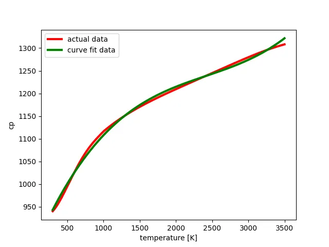
Explaining if the results are good or bad

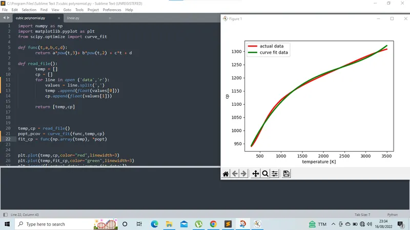
by using the cubic polynomial it has a minor difference in the plot so it does not has a lot of variation in the points so it can be used as a governing equation

Main Window

5. What needs to be done in order to make the curve fit perfect?

• We can make the curve fit better by either using a higher order polynomial or by breaking the temperature into two different ranges or both .
• the mathematical curve has some variation from the original curve it means it has some errors in the values of variables (a,b,c,d) in the equations considered.those values are not matching the original values that it should be .

6. Show empirically as to how well your curve has been fit.

By observation, a cubic predicted curve has been almost fit into original data curve with some tolerance compared to linear predicted curve. If curve fit overlapped to original data with comes under the defined some tolerances, it is called best fit.