Week 5 - Curve fitting
Curve Fitting using PYTHON
Objective -
There are two objectives :-
- To fit a linear and cubic polynomial for a given data and to get a best fit out of the two fits
- To get a perfect curve fit
Theory:-
lntroduction of curve Fitting Method :-
Curve fitting is a process of determining a best possible curve for a given data. This method is useful for extrapolation or interpolation of data. In simple words,curve fitting process can be used to find a data outside the given range.
There are various types of curve fitting process and the use of these process depends on the type of data given. Some of them are as follows -
- Linear Curve Fitting (Fitting of first order polynomial to a data)
- Cubic Curve Fitting (Fitting of third order polynomial to a data)
- Higher Order Curve Fitting (Fitting of higher order polynomial to a data)
- Curve Fitting using a Splitwise Polynomial Method (Using different/same order polynomial for the different divisions (parts) of given data range)
Parameters used to measure the fitness characteristics for the curve :-
There are four characteristics used to measure the fitness of the curve -
1. SSE (sum of Sqaured Errors) - It is the sum of square of the errors(i.e difference between individual values).For example,there is dataset with n points having individual error and assuming the best f it for the dataset to be y = f(x).
The error for general T point can be given by the function:
Error = ly(i) - value of f (x) at x(i)l = ly(i) - f(x(i))l
In order to remove the modulus sign we have to square the error term.So,squaring each error and adding them gives error for complete dataset.

Fit with value of SSE closer to zero indicates that the model has a smaller random error component, and that the fit will be more usef ulfor prediction.
2.R-square - It is the square of the corelation between original and predicted response values. It is the quantity that measures how successful is the fit in explaining the variation of the data.
R-square for the dataset with assumed fit as y = f(x),
R-square or R^2 = SSR/SST

Mean - arithmetic mean of the dataset
SST = SSR + SSE
Value of R-square varies from 0 to 1.
0 for worst possible fit for the data set and Ifor best possible fit for the data set.
Fit with value of R-square closer to Iindicating that a greater proportion of variance is accounted for by the model and indicating it is a better fit.
3.Adjusted R-square - It is a normalizing variation of R-square which neglects the variation of R-square due to insignificant independent variable
If value of x(i) contribute to the o/p y,then x(i) is a significant independent variable and if value of x(i) does not contribute to the o/p y,then x(i) is an insignificant independent variable.
Adjusted R-square = 1-(((1 - R-square)*(n - 1))/ (n - k - 1))
where, n - no of datapoints
k - number of independent variables
The adjusted R-square statistic can take on any value less than or equal to I,with a value closer to Iindicating a better fit. Negative values can occur when the modelcontains terms that do not help to predict the response.
4. RMSE (Root Mean Squared Error) - Also known as the fit standard error and the standard error of the regression.It is an estimate of the standard deviation of the random component in the data,and is defined as

where,n - no of datapoints
RMSE value closer to 0 indicates a fit that is more useful for prediction and indicates that it is a better fit.
Problem Statement -
1. What does popt and pcov mean? (Watch the video to get some context)
2. What does np.array(temperature) do?
3. What does the * in *popt mean?
4. Write code to fit a linear and cubic polynomial for the Cp data. Explain if your results are good or bad.
5. What needs to be done in order to make the curve fit perfect?
6. Show empirically as to how well your curve has been fit.
Solution of the P-roblem -
- Answer to Question Number 1
'popt' and 'pcov' are the output arguments of the Python's inbuilt function 'curve_fit' imported from 'scipy' module.
'popt' - First output argument i.e ·popt is a 2D array which consists the optimal(best fit) values of coefficients of a polynomial,used for curve fitting process,for which the sum of squared residuals for a given data is minimized.'popt' can be used to extract the coefficients of a polynomial.
'pcov' - Second output argument i.e 'pcov' is also a 2D array which gives an estimated values of covariance of coefficients (popt) of a polynomial. The diagonal elements of an array/matrix gives the value of covariance of a coefficient with itself which is also called as variance of that coefficent. Other non-diagonal elements of the matrix gives the covariance of a coefficient with other coefficient. It is a square matrix (no. of rows = no.of columns). This array/matrix indicates the uncertainities and correlation between the coefficients of a polynomialandit is mostly useful when the data has uncertainities.'pcov' can be used to find the standard deviation (square root of the value of diagonal elements) of a given dataset.
- Answer to Question Number 2
The command 'np.array(temperature)' is used for accessing the individual elements of the temperature array with the help of numpy module.Numpy module/ library is imported as 'np' and used to perform mathematicaloperations like addition,subtraction,multiplication,division,etc.on each element of an array or between the arrays.
- Answer to Question Number 3
The star i.e ., * in "popt' unpacks the 'popt' array so that the optimized coefficients (parameters) values can be accessed from the array 'popt'.In other words, · ·(* means all) aids in referring to all the values stored inthe array 'popt'.
- Answer to Question Number 4
Code to fit a linear and cubic polynomial to a cpdata :-
#Program to perform curve fitting using linear and cubic polynomial
#Importing the basic libraries/modules
import math
import matplotlib.pyplot as plt
import numpy as np
from scipy.optimize import curve_fit


#Function defined for reading the data file containing temperature and cp values
def read_file():
        temperature=[]
        cp = []
        #For loop for reading the file line by line and preparing the data
        for line in open ('data ','r'):
                values = line.split(',')
                temperature.append(float(values[0]))
                cp.append(float(values[1]))

        return [temperature, cp]
#Calling the function read_file to get temperature and cp values temperature, cp = read_file()
#Performing Curve Fitting using linear Polynomial
#Function to define the linear polynomial for curve fitting
def linear(T, a, b):
        return (a*T + b)

"""
linear Polynomial
cp = a*T + b
"""
popt1, pcov1 = curve_fit(linear, temperature, cp)
linear_fit_cp = linear(np.array(temperature), *popt1)

#Maximum Percentage Error
error1 = (np.array(np .array(cp)- np .array(linear_fit_cp)))*100/(np .array(cp))
max_error1 = max(error1)
print('Maximum Percentage Error for Curve Fitting using linear Polynomial = ', max_error1)
print('\n')

#Comparing original data with curve fit using linear polynomial

#Creating an empty figure window
plt.figure(1)
#Creating a plot
plt.plot(temperature, cp, color = 'r', linewidth = 2, label='Original Data')
plt.plot(temperature, linear_fit_cp, color = 'b', linewidth=2, label = 'Curve Fit')
#Giving a title to the plot
plt.title('Comparison of original data set and curve fit using linear polynomial ', color ='k', fontsize=15)

# Giving labels to the axes
plt.xlabel('Temperature [K]', fontsize = 12)
plt.ylabel('Specific Heat [kJ/kg-K]', fontsize=12)

#Inserting a legend
plt.legend (loc = 'lower right')
#Inserting the text in a plot
plt.text(500, 1280, 'Polynomial Equation : cp=' + str(popt1[0]) + '*T +' + str(popt1[1]),color='r',fontsize=10)
plt.text(500, 1250, 'Maximum Percentage Error=' +  str(max_error1)+ '%' , color = 'r', fontsize = 10)
# Saving the plot as an image in PNG format
plt.savefig('Curve fit using linear polynomial.png ')
# Making the plots visible
plt.show()
#Performing Curve Fitting using Cubic Polynomial
#Function to define the cubic polynomial for curve fitting
def cubic(T, a, b, c, d ):
        return (a*pow(T, 3)+ b*pow(T, 2)+ c*T + d)
"""
Cubic Polynomial
cp = a*TA3 + b*TA2 + c*T + d
"""

popt2, pcov2=curve_fit(cubic, temperature, cp)
cubic_fit_cp=cubic(np .array(temperature), *popt2)
#Maximum Percentage Error
error2 = (np.array(np.array(cp)- np.array(cubic_fit_cp)))*100/(np .array(cp))
max_error2 = max(error2)
print('Maximum Percentage Error for Curve Fitting using Cubic Polynomial = ', max_error2)
#Comparing original data i.ith curve fit using cubic polynomial
 #Creating an empty figure window
plt.figure(2)
#Creating a plot
plt.plot(temperature, cp, color = 'r', linewidth = 2, label = 'Original Data')
plt.plot(temperature, cubic_fit_cp, color = 'b ', linewidth = 2, label = 'Curve Fit')
#Giving a title to the plot
plt.title('Comparison of original data set and curve fit using cubic polynomial', color	='k', fontsize= 15)
# Giving labels to the axes
plt.xlabel('Temperature [K]', fontsize = 12)
plt.ylabel('Specific Heat [kJ/kg-K]', fontsize=12)

#Inserting a legend
plt.legend (loc ='lower right')
#Inserting the text in a plot
plt.text(200, 1280, 'Polynomial Equation : cp=' + str(popt2[0])+ '*T^3 +' + '('+str(popt2[1])+ ')' + '*T^2' + '('+str(popt2[2])+ ')' + '*T' + '('+str(popt2[3]))
plt.text(200, 1250, 'Maximum Percentage Error=' + str(max_error2)+ '%' , color = 'r', fontsize = 8)
 # Saving the plot as an image in PNG format
plt.savefig('Curve fit using cubic polynomial.png ')
# Making the plots visible
plt.show()Explanation of the code :-
- Import the basic modules like math,matploltib,numpy and scipy The math module is usedif any mathematical constants or trigonometric identities are used inthe program.The matplotlib module is used for plotting the graphs and numpy module is used to perform mathematical operations on the elements of the array (if any).The scipy module is used to perform curve fit operation by importing it as a optimization function.
- Defining the function 'read_file' which is further called for reading the thermodynamic data file line by line using the 'for' loop with 'line' as a counter variable and storing the data i.e temperature and spec if ic heat into two arrays 'temperature' and 'cp' respectively after splitting each line using the command 'linsplit(',')' where line is the variable having string format containing the data from each line and comma(,),the delimeter,used as a seperator.
- The function 'read_file' is called then to get the arrays 'temperature' and 'cp'.
- Function named as 'linear' is used to define the linear polynomialwhich is aim to be fitted to the data.
- 'popt' (best fit value of coefficients) and 'pcov'(estimated va lue of covariance of coefficients) are obtained as output arguments by calling the Python's inbuilt function named as 'curve_fit' and passing the function named as 'linear' and the arrays 'temperature' and 'cp' inside the function 'curve_fit' as an input arguments. Then,the new value of cp according to the linear polynomial i.e 'linear _fit_cp' is calculated by calling the function 'linear' (defined earlier) and passing 'temperature' array element wise using numpy module and allthe coefficients of the linear polynomial using '*popt' as an input arguments.
- Maximum percentage error is calculated by extracting the maximum va lue from the array 'error'which is calculated using the arrays 'cp' and 'linear_fit_cp'. It is printed in the command window using the command 'print()'.
- A figure of compsarison is obtained by plotting the original dataset plot i.e (temperature vs cp) and the curve fit plot i.e (temperature vs linear_ f it_cp) ina single f igure win Also,the text like polynomialequation and maximum percentage error is inserted in the f igure window using the command 'pit.text'.
- Similarly,the cubic polynomialis fitted to the data except the fourth step in which a cubic polynomial is defined which is further passed as an input argument inside the 'curve_fit' function and used for calculating the new value of cp i.e 'cubic_f it_cp'. Also,a figure of comparison is obtained by plotting the original dataset plot i.e (temperature vs cp) and the curve fit plot i.e (temperature vs cubic_fit_cp) in a single figure win
Output of the program :-
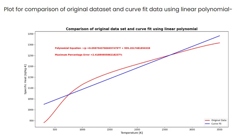
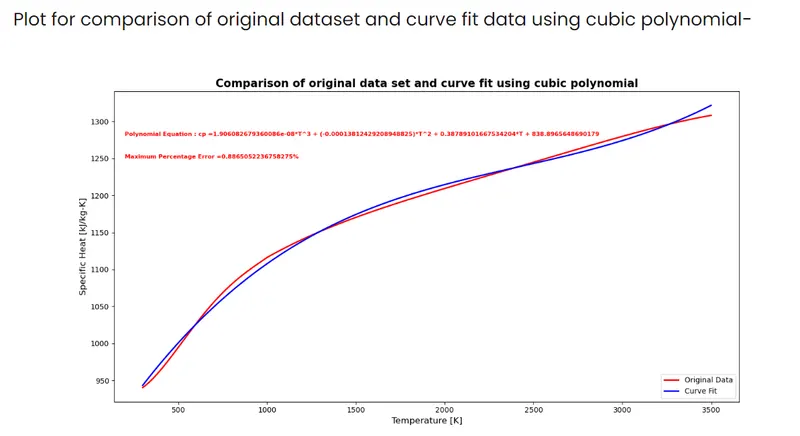
Maximum percentage error in command window for both cases are shown.
Comparison of fits for explanation of which results are better:-
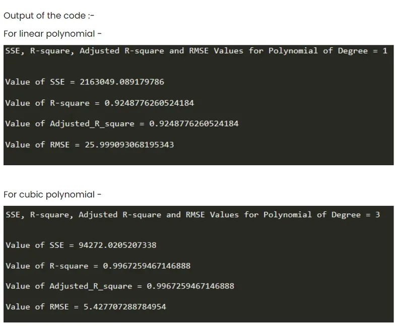
ln order to compare the fits,we need to observe the comporsion plots and we also have to calcuate and compare the R-square and RMS values for the two f its.The fit with value of RMS close to zero and value of R-square close to 1 is the best f it.
Code to calculate the R-square and RMS values for linear and cubic polynomial fit :-
#Program to calculate the fitness characteristics for curve fitting with linear and cubic polynomial
#Importing the basic libraries/modules
import math
import matplotlib.pyplot as plt
import numpy as np
from scipy.optimize import curve_fit

#Function defined for reading the data file containing temperature and cp values
def read_file():
        temperature=[]
        cp = []

        #For loop for reading the file line by line and preparing the data
        for line in open ('data ', 'r'):
            values = line.split(',')
            temperature.append(float(values[0]))
            cp.append(float(values[1]))

        return [temperature, cp]


#Calling the function read_file to get temperature and cp values
temperature, cp = read_file()
#Number of datapoints
n = len(temperature)

#Number of independent variables
k = 0
#Performing Curve Fitting using linear Polynomial

#Function to define the linear polynomial for curve fitting
def linear(T, a, b):
        return (a*T + b)

"""
linear Polynomial
cp = a*T + b
"""
popt1, pcov1 = curve_fit(linear, temperature, cp)
linear_fit_cp = linear(np.array(temperature), *popt1)
#Calculation of fitness characteristics

#Goodness of Curve Fit
print('SSE , R-square, Adjusted R-square and RMSE Values for Polynomial of Degree=	1')
print('\n')

#Sum of Square of Errors (SSE)
SSE = np.sum(pow((np .array(np .array(cp)- np .array(linear_fit_cp))), 2))
print('Value of SSE =', SSE)
print('\t')

# Sum of squares of regression (SSR)
SSR = np.sum(pow((np .array(np .array(linear_fit_cp)- np.mean(cp))), 2))
#Total sum of squares (SST)
SST = SSE + SSR
#R-square
R_square = SSR/SST
print('Value of R- square =' , R_square)
print('\t')

#Adjusted R-square
Adjusted_R_square = 1 - ((1 - R_square)*(n - 1)/(n - k - 1))
print('Value of Adjusted_R_square=',Adjusted_R_square)
print('\t')

#Root Mean Squared Error(RMSE)
RMSE = np.sqrt((np.sum(pow((np .array(np .array(cp)- np.array(linear_fit_cp))), 2)))/n);
print('Value of RMSE = ', RMSE)
print('\n')
print('\t')
#Performing Curve Fitting using Cubic Polynomial

#Function to define the cubic polynomial for curve fitting
def cubic(T, a, b, c, d ):
        return (a*pow(T, 3)+ b*pow(T, 2)+ c*T + d)
"""
Cubic Polynomial
cp = a*T^3 + b*T^2 + c*T + d
"""
popt2, pcov2=curve_fit(cubic , temperature, cp)
cubic_fit_cp=cubic(np .array(temperature), *popt2)
#Calculation of fitness characteristics
#Goodness of Curve Fit
print('SSE, R-square, Adjusted R-square and RNSE Values for Polynomial of Degree=3')
print('\n')

#Sum of Square of Errors (SSE)
SSE = np.sum(pow((np.array(np .array(cp)- np .array(cubic_fit_cp))), 2))
print('Value of SSE = ', SSE)
print('\t')
# Sum of squares of regression (SSR)
SSR = np.sum(pow((np.array(np.array(cubic_fit_cp)- np.mean(cp))), 2))
#Total sum of squares (SST)
SST = SSE + SSR

#R-square
R_square = SSR/SST
print ('Value of R- square =' , R_square)
print('\t')

#Adjusted R-square
Adjusted_R_square = 1 -((1 - R_square)*(n - 1)/(n - k - 1))
print ('Value of Adjusted_R_square = ', Adjusted_R_square)
print('\t')

#Root Mean Squared Error(RMSE)
RMSE = np.sqrt((np.sum(pow((np.array(np .array(cp)- np .array(cubic_fit_cp))), 2)))/n);
print('Value of RMSE = ', RMSE)
print('\n')
print('\t')
Explanation of results of a code to fit a linear and cubic polynomial to a cp data :-
By observing the above two plots for comparison of original dataset and curve f it data and seeing the results of the code to calculate the R-square and RMS values for linear and cubic curve fit (i.e the value of R-square and Adjusted R-square which is closer to 1 and value of SSE and RMSE which is closer to 0 for cubic curve fit as compared to the corresponding values for linear curve fit),we can conclude that results of the cubic curve f it are better than that of the linear curve f it. In other words,cubic curve fit is the best f it among the two curve fits.
5.Answer to Question Number 5
How to make a curve fit perfect/How to fit a curve perfectly :-
- Order of the polynomial can also be increased to get a pefect fi But inthis method we get a perfect curve for a polynomial having very high order.
Plot for compar ison of originaldataset and curve f it data are shown for various order polynomials are shown below -
a) 4th Order Polynomial -
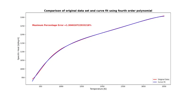
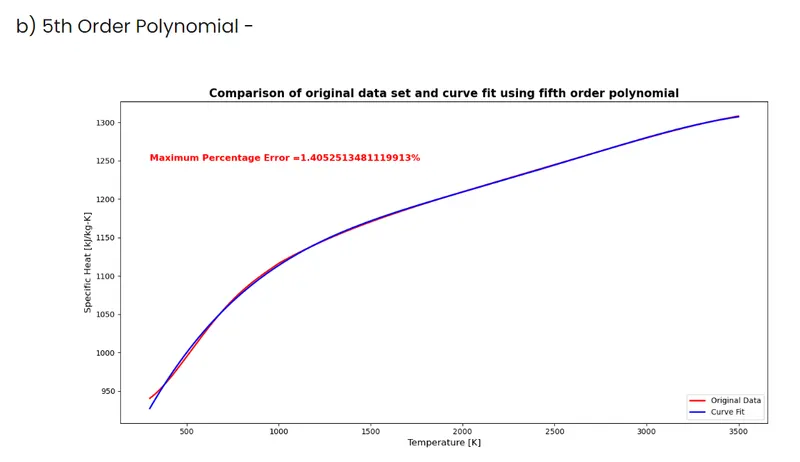
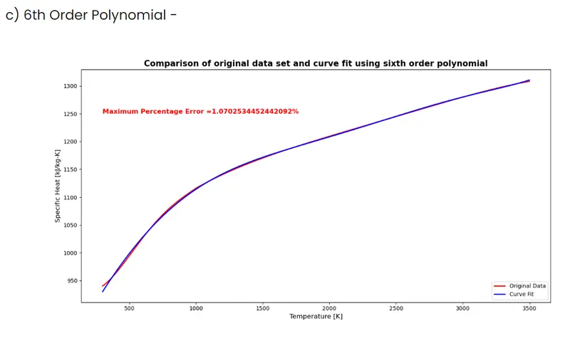
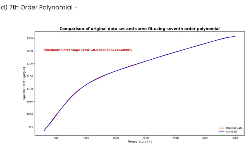
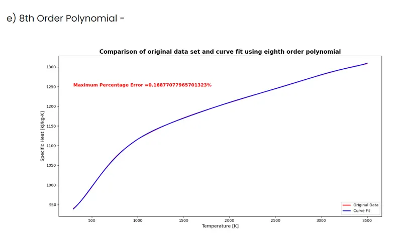
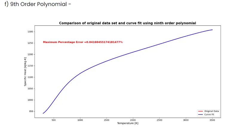
So,in order to get a perfect fit we have to use a 9th order polynomial.
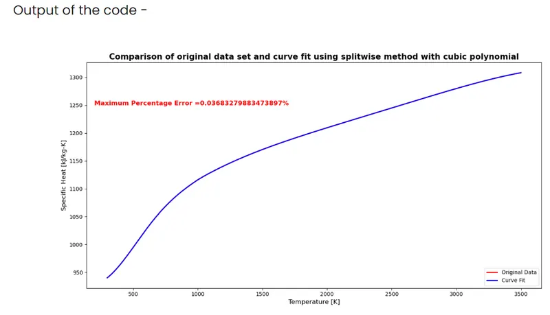
2.Another way to get a perfect f it is to use a splitwise polynomialmethod. In this method the temperature and specific heat data is splitted into parts. Curve fitting can be done by using similar or different degree polynomials to obtain a complete single curve.The advantage of this method over using higher order polynomialis that a perfect f it can be obtained by using lower order polynomial. Like in f igure below perfect f it is obtained by using a 3rd degree polynomial and having maximum percentage error equal to 0.0368327988% which is less as compared to 9thorder polynomial in the above case.
Code to perform splitwise method for curve fitting -
#Program to calculate the fitness characteristics for curve fitting with linear and cubic polynomial
#Importing the basic libraries/modules
import math
import matplotlib.pyplot as plt
import numpy as np
from scipy.optimize import curve_fit


#Function defined for reading the data file containing temperature and cp values
def read_file():
        temperature=[]
        cp = []
        #For loop for reading the file line by line and preparing the data
        for line in open ('data ','r'):
            values = line.split(',')
            temperature.append(float(values[0]))
            cp.append(float(values[1]))

        return [temperature, cp]
#Calling the function read_file to get temperature and cp values
temperature, cp = read_file()
#Preparing the temperature and cp arrays for 8 different ranges
#Temperature and cp values for Range[1 - 400]
temperature1 = temperature[0:400]
cp1 = cp[0:400]
#Temperature and cp values  for Range[401 - 800]
temperature2 = temperature[400:800]
cp2 = cp[400:800]

#Temperature and cp values for Range[801 - 1200]
temperature3 = temperature[800:1200]
cp3 = cp[800:1200]

#Temperature and cp values for Range[1201 - 1600]
temperature4 =  temperature[1200:1600]
cp4 = cp[1200:1600]
#Temperature and cp values for Range[1601 - 2000]
temperatures =  temperature[1600:2000]
cp5 = cp[1600:2000]
#Temperature and cp values for Range[2001 - 2400]
temperature6 =  temperature[2000:2400]
cp6 = cp[2000:2400]
#Temperature and cp values for Range[2401 - 2800)
temperature7 =  temperature[2400:2800]
cp7 = cp[2400:2800]

#Temperature and cp values for Range[2801 - 3200]
temperatures = temperature[2800:3200]
cp8 = cp[2800:3200]

#Performing Curve Fitting using Cubic Polynomial for all ranges in splitwise method

#Function to define the cubic polynomial for curve fitting for splitwise method
def cubic(T, a, b, c, d):
        return (a*pow(T, 3)+ b*pow(T, 2)+ c*T + d)
#Curve Fitting for all Ranges
#Range(1 - 400)
popt1, pcov1 =  curve_fit(cubic, temperature1, cp1)
splitwise_cubic_fit_cp1 = cubic(np.array(temperature1), *popt1)

#Range(401 - 800)
popt2, pcov2 = curve_fit(cubic, temperature2, cp2)
splitwise_cubic_fit_cp2 = cubic(np.array(temperature2), *popt2)

#Range(801 - 1200)
popt3, pcov3 = curve_fit(cubic, temperature3, cp3)
splitwise_cubic_fit_cp3 = cubic(np.array(temperature3), *popt3)

#Range(1201 - 1600)
popt4, pcov4 = curve_fit(cubic,temperature4, cp4)
splitwise_cubic_fit_cp4 =cubic(np.array(temperature4), *popt4)

#Range(1601 - 2000)
popt5, pcov5 = curve_fit(cubic,temperatures, cps)
splitwise_cubic_fit_cp5 =cubic(np.array(temperature5), *popt5)

#Range(2001 - 2400)
popt6, pcov6 = curve_fit(cubic, temperature6, cp6)
splitwise_cubic_fit_cp6 = cubic(np.array(temperature6), *popt6)

#Range(2401 - 2800)
popt7, pcov7 = curve_fit(cubic, temperature7, cp7)
splitwise_cubic_fit_cp7 = cubic(np.array(temperature7), *popt7)

#Range(2801 - 3200)
popt8, pcov8 = curve_fit(cubic, temperatures, cp8)
splitwise_cubic_fit_cp8 = cubic(np.array(temperature8), *popt8)
#Creation of spliti.ise_cubic_fit_cp array
splitwise_cubic_fit_cp  =  np.concatenate((splitwise_cubic_fit_cp1, splitwise_cubic_fit_cp2, splitwise_cubic_fit_cp3,splitwise_cubic_fit_cp4,splitwise_cubic_fit_cp5,splitwise_cubic_fit_cp6,splitwise_cubic_fit_cp7,splitwise_cubic_fit_cp8))

#Maximum Percentage Error
error = (np.array(np.array(cp)- np.array(splitwise_cubic_fit_cp)))*100/(np.array(cp))
max_error = max(error)


#Comparing original data with curve fit using splitwise method >iith cubic polynomial

#Creating an empty figure window
plt.figure()

#Creating a plot
plt.plot(temperature, cp, color = 'r', linewidth = 2, label = 'Original Data')
plt.plot(temperature, splitwise_cubic_fit_cp, color = 'b ', linewidth = 2, label='Curve Fit')

#Giving a title to the plot
plt.title('Comparison of original data set and curve fit using splitwise method with cubic polynomial', color='b', fontsize=12)
# Giving labels to the axes
plt.xlabel('Temperature [K]', fontsize = 12)
plt.ylabel('Specific Heat [kJ/kg-K]', fontsize=12)
#Inserting a legend
plt.legend (loc = 'lower right')
#Inserting the text in a plot
plt.text(200, 1250, 'Maximum Percentage Error=' +  str(max_error)+ '%' , color='r' , fontsize=12)
# Saving the plot as an image in PNG format
plt.savefig('Curve fit using splitwise method with cubic polynomial.png')
# Making the plots visible
plt.show()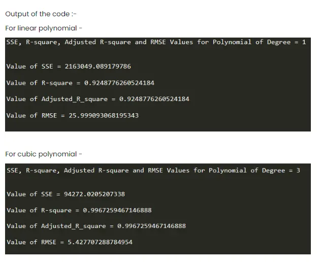
Explanation of results of a code to fit a linear and cubic polynomial to a cp data :-
By observing the above two plots for comparison of original dataset and curve f it data and seeing the results of the code to calculate the R-square and RMS values for linear and cubic curve fit (i.e the value of R-square and Adjusted R-square which is closer to 1 and value of SSE and RMSE which is closer to 0 for cubic curve f it as compared to the corresponding values for linear curve fit),we can conclude that results of the cubic curve fit are better than that of the linear curve f it. In other words,cubic curve fit is the best f it among the two curve fits.
5.Answer to Question Number 5
How to make a curve fit perfect/How to fit a curve perfectly :-
- Order of the polynomial can also be increased to get a pefect fi But inthis method we get a perfect curve for a polynomial having very high order.
Plot for compar ison of originaldataset and curve f it data are shown for various order polynomials are shown below -
- a) 4th Order Polynomial -
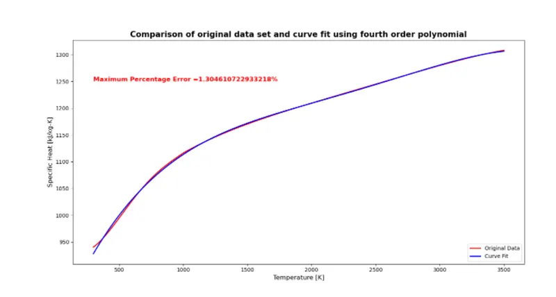
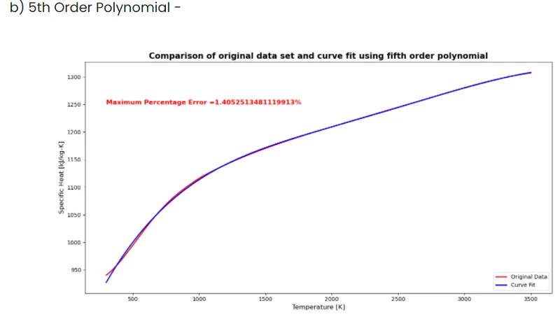
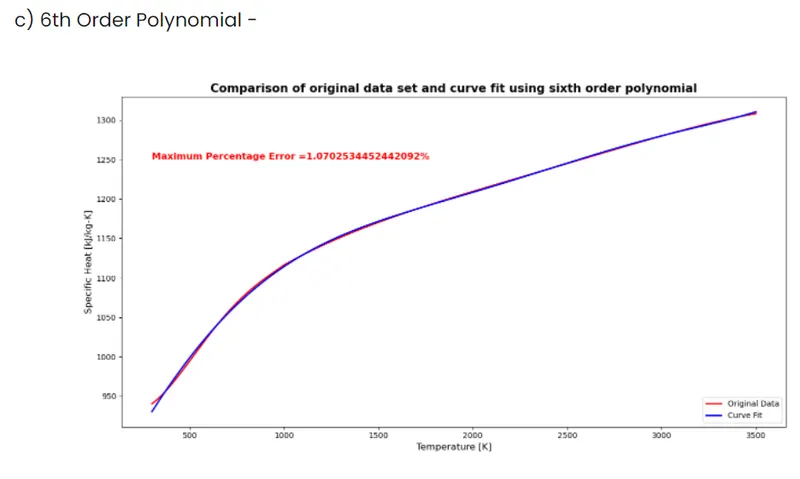
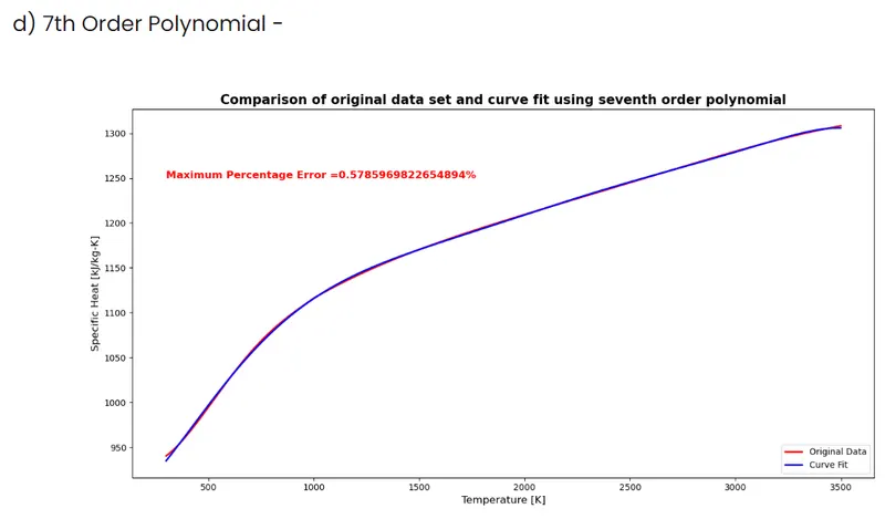
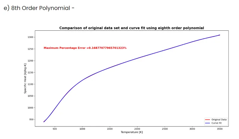
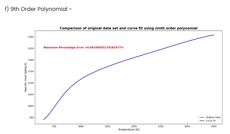
So,in order to get a perfect f it we have to use a 9thorder polynomial.
- Another way to get a perfect f it is to use a splitwise polynomialmethod. In this method the temperature and
specif ic heat data is splitted into parts. Curve fitting can be done by using similar or different degree polynomials to obtain a complete single curve.The advantage of this method over using higher order polynomialis that a perfect f it can be obtained by using lower order polynomial. Like in f igure below perfect f it is obtained by using a 3rd degree polynomial and having maximum percentage error equal to 0.0368327988% which is less as compared to 9thorder polynomial in the above case.
Code to perform splitwise method for curve fitting -
#Program to calculate the fitness characteristics for curve fitting with linear and cubic polynomial
#Importing the basic libraries/modules
import math
import matplotlib.pyplot as plt
import numpy as np
from scipy.optimize import curve_fit


#Function defined for reading the data file containing temperature and cp values
def read_file():
        temperature=[]
        cp = []
        #For loop for reading the file line by line and preparing the data
        for line in open ('data ','r'):
            values = line.split(',')
            temperature.append(float(values[0]))
            cp.append(float(values[1]))

        return [temperature, cp]
#Calling the function read_file to get temperature and cp values
temperature, cp = read_file()
#Preparing the temperature and cp arrays for 8 different ranges
#Temperature and cp values for Range[1 - 400]
temperature1 = temperature[0:400]
cp1 = cp[0:400]
#Temperature and cp values  for Range[401 - 800]
temperature2 = temperature[400:800]
cp2 = cp[400:800]

#Temperature and cp values for Range[801 - 1200]
temperature3 = temperature[800:1200]
cp3 = cp[800:1200]

#Temperature and cp values for Range[1201 - 1600]
temperature4 =  temperature[1200:1600]
cp4 = cp[1200:1600]
#Temperature and cp values for Range[1601 - 2000]
temperatures =  temperature[1600:2000]
cp5 = cp[1600:2000]
#Temperature and cp values for Range[2001 - 2400]
temperature6 =  temperature[2000:2400]
cp6 = cp[2000:2400]
#Temperature and cp values for Range[2401 - 2800)
temperature7 =  temperature[2400:2800]
cp7 = cp[2400:2800]

#Temperature and cp values for Range[2801 - 3200]
temperatures = temperature[2800:3200]
cp8 = cp[2800:3200]

#Performing Curve Fitting using Cubic Polynomial for all ranges in splitwise method

#Function to define the cubic polynomial for curve fitting for splitwise method
def cubic(T, a, b, c, d):
        return (a*pow(T, 3)+ b*pow(T, 2)+ c*T + d)
#Curve Fitting for all Ranges
#Range(1 - 400)
popt1, pcov1 =  curve_fit(cubic, temperature1, cp1)
splitwise_cubic_fit_cp1 = cubic(np.array(temperature1), *popt1)

#Range(401 - 800)
popt2, pcov2 = curve_fit(cubic, temperature2, cp2)
splitwise_cubic_fit_cp2 = cubic(np.array(temperature2), *popt2)

#Range(801 - 1200)
popt3, pcov3 = curve_fit(cubic, temperature3, cp3)
splitwise_cubic_fit_cp3 = cubic(np.array(temperature3), *popt3)

#Range(1201 - 1600)
popt4, pcov4 = curve_fit(cubic,temperature4, cp4)
splitwise_cubic_fit_cp4 =cubic(np.array(temperature4), *popt4)

#Range(1601 - 2000)
popt5, pcov5 = curve_fit(cubic,temperatures, cps)
splitwise_cubic_fit_cp5 =cubic(np.array(temperature5), *popt5)

#Range(2001 - 2400)
popt6, pcov6 = curve_fit(cubic, temperature6, cp6)
splitwise_cubic_fit_cp6 = cubic(np.array(temperature6), *popt6)

#Range(2401 - 2800)
popt7, pcov7 = curve_fit(cubic, temperature7, cp7)
splitwise_cubic_fit_cp7 = cubic(np.array(temperature7), *popt7)

#Range(2801 - 3200)
popt8, pcov8 = curve_fit(cubic, temperatures, cp8)
splitwise_cubic_fit_cp8 = cubic(np.array(temperature8), *popt8)
#Creation of spliti.ise_cubic_fit_cp array
splitwise_cubic_fit_cp  =  np.concatenate((splitwise_cubic_fit_cp1, splitwise_cubic_fit_cp2, splitwise_cubic_fit_cp3,splitwise_cubic_fit_cp4,splitwise_cubic_fit_cp5,splitwise_cubic_fit_cp6,splitwise_cubic_fit_cp7,splitwise_cubic_fit_cp8))

#Maximum Percentage Error
error = (np.array(np.array(cp)- np.array(splitwise_cubic_fit_cp)))*100/(np.array(cp))
max_error = max(error)


#Comparing original data with curve fit using splitwise method >iith cubic polynomial

#Creating an empty figure window
plt.figure()

#Creating a plot
plt.plot(temperature, cp, color = 'r', linewidth = 2, label = 'Original Data')
plt.plot(temperature, splitwise_cubic_fit_cp, color = 'b ', linewidth = 2, label='Curve Fit')

#Giving a title to the plot
plt.title('Comparison of original data set and curve fit using splitwise method with cubic polynomial', color='b', fontsize=12)
# Giving labels to the axes
plt.xlabel('Temperature [K]', fontsize = 12)
plt.ylabel('Specific Heat [kJ/kg-K]', fontsize=12)
#Inserting a legend
plt.legend (loc = 'lower right')
#Inserting the text in a plot
plt.text(200, 1250, 'Maximum Percentage Error=' +  str(max_error)+ '%' , color='r' , fontsize=12)
# Saving the plot as an image in PNG format
plt.savefig('Curve fit using splitwise method with cubic polynomial.png')
# Making the plots visible
plt.show()