Week 5 - Curve fitting

AIM:

To write a program for a perfect Curve fit using Python.

1. What does popt and pcov mean?

• the popt calculates the values of a and b (1), from the above command the curve fit function returns 2 items which we call popt and pcov.
• the best curve fit parameters for the variables a and b is assigned in the popt argument.
• the uncertainites and correlations between parameters is indicated by the pcov variable which stores the voariance matrix.

2. What does np.array(temperature) do?

• Numpy arrays provide the dimensional attribute that returns an integer that tells u how many dimension contained in the array.

3. What does the * in *popt mean?

• the popt is an array of optimal values of constraints in the function and * asterick refers to the address of all the constraints.

4. Write code to fit a linear and cubic polynomial for the Cp data.

Python Program:

# python program for Curve Fit.
# Program by Simeon T

# importing essential library tools
import math  						  # importing math library tools 
import matplotlib.pyplot as plt 	  # importing plotting library tools
import numpy as np  				  # importing numberical and logical libraty tools
import scipy as sp  				  # importing scientific library tools
from scipy.optimize import curve_fit  # importing the curve fit library tools

# Defining the linear function
def func(t,a,b):  # defining the function
	return a*t+b  # returning the function
 
# reading the thermodynamic data
def read_file():  							  # preparing the data
	temperature=[]  						  # storing temperature data 
	cp=[] 									  # storing the specific heat 
	for line in open('data','r'):  	 		  # openning the given data and declaring in the loop
		values=line.split(',') 				  # spliting the values with reference with comma
		temperature.append(float(values[0]))  # attaching the temperatures along with the loop
		cp.append(float(values[1]))  		  # attaching the specific heat along with the loop
	return[temperature,cp]       			  # returning the temperature and Specific heat values

temperature,cp=read_file()  			  # defining temperature along with the read file temperature
popt,pcov=curve_fit(func,temperature,cp)  # declaring popt, pcov as a function of curve fit
cp_fit=func(np.array(temperature),*popt)  # defining the curve fit as a function of popt
print(popt)                               # printing the popt

# plotting the curve
plt.figure(1)  
plt.grid()
plt.plot(temperature,cp,color='red')
plt.plot(temperature,cp_fit,color='green')
plt.legend(['Actual data','Quadratic Curve Fit'])
plt.xlabel('temperature in K')
plt.ylabel('specific heat at cp')
plt.show()

# Cubic fit function
def func(t,a,b,c,d):  					 # defining the function
	return a*pow(t,3)+b*pow(t,2)+c*t+d   # returning the function

# reading the thermodynamic data
def read_file():  							   # preparing the data
	temperature=[]   						   # storing temperature data 
	cp=[]  									   # storing the specific heat 
	for line in open('data','r'):   		   # openning the given data and declaring in the loop
		values=line.split(',')  			   # spliting the values with reference with comma
		temperature.append(float(values[0]))   # attaching the temperatures along with the loop
		cp.append(float(values[1]))            # attaching the specific heat along with the loop
	return [temperature,cp]                    # returning the temperature and Specific heat values 

temperature,cp=read_file()   			  # defining temperature along with the read file temperature
popt,pcov=curve_fit(func,temperature,cp)  # declaring popt, pcov as a function of curve fit
cp_fit=func(np.array(temperature),*popt)  # defining the curve fit as a function of popt
print(popt)                               # printing the popt

# plotting
plt.figure(2)
plt.grid()
plt.plot(temperature,cp,color='blue')
plt.plot(temperature,cp_fit,color='green')
plt.legend(['Actual data','Cubic Curve Fit'])
plt.xlabel('temperature in K')
plt.ylabel('specific heat at cp')
plt.show()

# end

Explanation:

• STEP 1: Importing libraries
  
  • in this step we will first import all the required library tools like math, scipy, numpy and matplotlib and from scipy we will be importing the curve fit.
• STEP 2 : Defining the function.
  
  • defining th function for th polynomial in whihc at first we will take all the variable and constants.
  • then we will read the data file available in the question and import the temperature and specific value.
  • first we will read the data file abd then we will find out the constant value of the polynomial equation.
• STEP 3: Finding the perfect fit
  
  • in order to make perfect fit, we must consider error estimates as well.
  • using the functions we will be getting the error percentage.
• STEP 4: plotting
  
  • After the functions are defined we will be priniting the results and plotting the same in the figure,

Explain if your results are good or bad.

• The plot is not so satisfying because the orginal curve of the observed data looks like of quadratic or cubic nature.
• The linear curve has a lot of variation in comparision to the actual curve, so the results needs to be improved and linear equation is not the fit.

5. What needs to be done in order to make the curve fit perfect?

• The curve should fit the orginal curve without showing any errors( such as centering and scaling errors) in that particular degree of polynomial, in order to make perfect fit, we must consider error estimates as well.

6. Show empirically as to how well your curve has been fit.

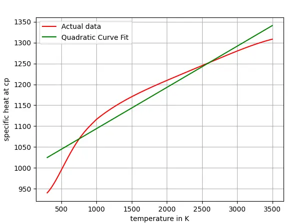
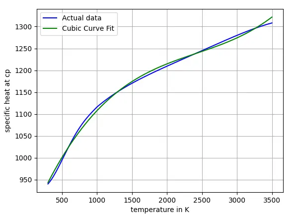
• from the above graphs we can see the results obtained for the linear curve vs actual data file and temperature, cp.
• the cubic curve vs actual data file between temperatire and cp.
• the perfect cubic curve is the 2nd image.

Error:

temperature.append(float(values[]))
^
SyntaxError: invalid syntax

RESULT:

Thus the program for a perfect Curve fit using Python is completed successfully and the output is verified.