Week 5 - Curve fitting

Curve fitting:

Curve fitting is the process of constructing a curve, or mathematical function, that has the best fit to a series of data points, possibly subject to constraints. Curve fitting can involve either interpolation, where an exact fit to the data is required, or smoothing, in which a "smooth" function is constructed that approximately fits the data.

1. What does popt and pcov mean?

poptarray

Optimal values for the parameters so that the sum of the squared residuals of f(xdata, *popt) - ydata is minimized.

pcov2-D array

The estimated covariance of popt. The diagonals provide the variance of the parameter estimate. To compute one standard deviation errors on the parameters use perr = np.sqrt(np.diag(pcov)).

How the sigma parameter affects the estimated covariance depends on absolute_sigma argument, as described above.

If the Jacobian matrix at the solution doesn’t have a full rank, then ‘lm’ method returns a matrix filled with np.inf, on the other hand ‘trf’ and ‘dogbox’ methods use Moore-Penrose pseudoinverse to compute the covariance matrix.

2. What does np.array(temperature) do?

This command is used to convert the all temperature into the numpy function , this command is used for some of the math operation cannot be done on list.

3. What does the * in *popt mean?

There is a way to simplify the call to the function with the best-fit parameters, which is:

• line(x, *popt)
  The * notation will expand a list of values into the arguments of the function. This is useful if your function has more than one or two parameters.
  Secondary and third array also we used for cubic curve fit.

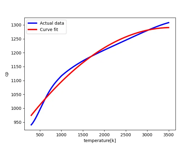
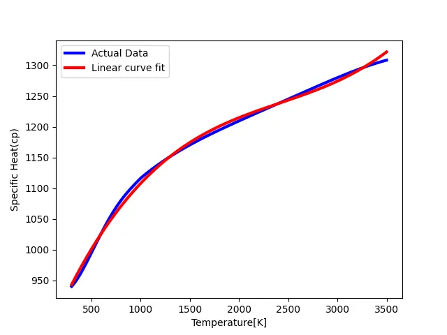
4. Write code to fit a linear and cubic polynomial for the Cp data. Explain if your results are good or bad.

• Curve fitting (Linear polynomial):

import numpy as np
import matplotlib.pyplot as plt
from scipy.optimize import curve_fit
from scipy.sparse import data

#curve fit function
def func(t, a, b, c):
    return a*pow(t,2) + b*t + c

#reading thermodynamic data file
def read_file():
    temperature = []
    cp = []
    for line in open('data','r'):
        values = line.split(',')
        temperature.append(float(values[0]))
        cp.append(float(values[1]))
    return [temperature, cp]

#main program
temperature, cp = read_file()
popt , pcov = curve_fit(func, temperature, cp)
fit_cp = func(np.array(temperature), *popt)

plt.plot(temperature, cp,color ="blue",linewidth =3)
plt.plot(temperature, fit_cp, color ="red", linewidth =3)
plt.legend(['Actual data', 'Curve fit'])
plt.xlabel('temperature[k]')
plt.ylabel('cp')
plt.show()

• Curve fitting (Cubic Polynomial):

import matplotlib.pyplot as plt
import numpy as np
from scipy.optimize import curve_fit

#curve fit function (Cubic)
def func(t,a,b,c,d):
    return a*pow(t,3)+b*pow(t,2)+c*t+d

##reading thermodynamic data file
def read_file():
    temperature =[]
    cp = []
    for line in open('data','r'):
        value = line.split(',')
        temperature.append(float(value[0]))
        cp.append(float(value[1]))
    return[temperature,cp]

#main program
temperature,cp =read_file()
popt,pcov = curve_fit(func,temperature,cp)
fit_cp = func(np.array(temperature),*popt)
print(popt)
plt.plot(temperature,cp,color ="blue",linewidth="3")
plt.plot(temperature,fit_cp,color="red",linewidth ="3")
plt.legend(['Actual Data','Linear curve fit'])
plt.xlabel('Temperature[K]')
plt.ylabel('Specific Heat(cp)')
plt.savefig('Linear curve fit')
plt.show()

• Procedure:
  Importing the required files for program running like "matplotlib","numpy","scipy for curve fit".
• Defining the Linear order equation(a*t+b) for the running linear polynomial .
• Creating a empty array for for the temperature and specific heat ,cp used to stored the values .
• Using for loop command in which it used for line to open ('data','r'), which is used to read the content of the data in which we read.
• Using command value =line.split(','), which is used to split the data as we required.
• Data we used to string value used convert with float and append command used to store the value in empty array we created.
• By using the "curve_fit" function fpr linear order, we get an output for temperature and specific heat cp.
• After getting the output as an popt , the output value of fit_cp we pass the value of temperature in data as numpy array so that it can be executed.
• We need to plot the output data using the plt.plot of temperature and specific heat cp & temperature with fit_cp.
• After finishing the case 1, for case 2 we need to use the cubic order of equation a*pow(t,3)+b*pow(t,2)+c*t+d
• And rest of the procedure are same as the above method.

Output:

• Linear function Output:

• Cubic function output:

5. What needs to be done in order to make the curve fit perfect?

From tha above two methods shows that while using the higher order equation , we will get the accurate result according to the data we have , so its suggest to use higher order equation for desired reault with minimum error.