Week 5 - Curve fitting

objective:to write a programm curvefitting wwith sets in linear and cubic fit

curvefitting can be defined as the process of a curve or mathamatical function

has the best fit to series of data points,subject to constraints.

the result obtained consists of the curve for specific heat as afunction of tempearture

will be comared with the actual plot.

the specific heat at different temperatures will be provided as inputs.

intially we have tio write the linear and cubic ploynomaial and check the results with actualplot

some important terms:

popt:it gives an array with the optimal values for the parameters so thatsum of the squared resuidals

of data is minimiozed

pcov:it is 2d array with the estimated covariance of the parameters in popt.it can be used to caliculate the

standard deviation errors of popt.

np.array(temperature):this function stores the values of temperature in the form of array and passes it in to function numpy

*in*popt:it stores the values of constant parametres (a,b,c) in the array plot.

for linearfit programm

import numpy as np 
import matplotlib.pyplot as plt 
from scipy.optimize import  curve_fit

#curve fit finction
def func(t,b,c):
	return b*t+c
#reading thermodynamic file
def read_file():
	temperature=[]
	cp=[]
	for line in open('data','r'):
		values=line.split(',')
		temperature.append(float(values[0]))
		cp.append(float(values[1]))

	return [temperature,cp]
#main program
temperature,cp=read_file()
popt,pcov=curve_fit(func,temperature,cp)
fit_cp=func(np.array(temperature),*popt)
#plotting values

plt.plot(temperature,cp,color="blue",linewidth=3)
plt.plot(temperature,fit_cp,color="red",linewidth=3)
plt.legend(['Actual data','curve fit'])
plt.xlabel('Temperature[k]')
plt.ylabel('cp')
plt.show()

for cubic fit programm

import numpy as np 
import matplotlib.pyplot as plt 
from scipy.optimize import  curve_fit

#curve fit finction
def func(t,a,b,c,d):
	return a*pow(t,3)+b*pow(t,2)+c*t+d
#reading thermodynamic file
def read_file():
	temperature=[]
	cp=[]
	for line in open('data','r'):
		values=line.split(',')
		temperature.append(float(values[0]))
		cp.append(float(values[1]))

	return [temperature,cp]
#main program
temperature,cp=read_file()
popt,pcov=curve_fit(func,temperature,cp)
fit_cp=func(np.array(temperature),*popt)
#plotting

plt.plot(temperature,cp,color="blue",linewidth=3)
plt.plot(temperature,fit_cp,color="red",linewidth=3)
plt.legend(['Actual data','curve fit'])
plt.xlabel('Temperature[k]')
plt.ylabel('cp')
plt.show()

code explanation

Code explanation:

• Importing useful libraries math,matplotlib,numpy and curvefit from scipy.optimize
• Define linear function
• Defining readfile
• Creating empty temperature array and cp
• Now open data file and read file
• Using linesplit sperate temp,cp lines
• Temperatue is indexed as 0 and cp as1
• Now return the value of temperature and cp backto funmction
• Curvefitting function has a attributes the function

result for linear

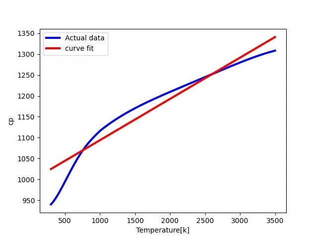
By using linear curve to fit the given data,the plot is not satisfying because the original curve

Of the observed curve looks like of quradratic or cubic nature.the linear curve has lot of variations

In camparision to the actual curve so results r=are bad by using a linear equation

result for cubicfit

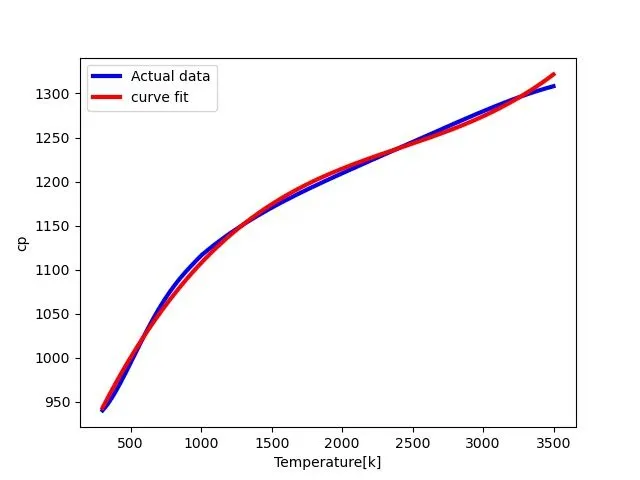
by using the cubic ploynomail it has minor difference in the plot so it does not has a lot of variations

result/observation:

it is clear from the above figures that the curve fits better when the degree of ploynomial increaes.it can be observed

the devaiation of the curve fit with the actual data is more for linear equation and gradually the deviation decreases

with the increase of the order of polynomial.

another method to get abetter fit could be using splitwise method