Week 5 - Curve fitting

Aim:

To prepare a Python code to perform Curve Fit for a given data sample.

Governing Equations:

Linear function - ax^2+bx+c

Cubic function - ax^3+bx^2+cx+d and so on,

For a better fit we can increase the no of polynomials.

Objective:

By using curve_fit function in python we need to get a best fit for the given data sample

Theory:

1. What does popt and pcov means?

When we use the curve_fit function we get two outputs which we named as popt and pcov.

Popt – popt stores optimal values for the equation of the curve, which would be the best fit for given polynomial. Suppose if we are using a linear polynomial popt would store values for a,b and c.

Pcov – pcov contains the covariance matrix. The variance in the fitted parameters represents the uncertainty in the best-fit value based on the quality of the fit of the model to the data. That is, it describes by how much the value could change away from the best-fit value and still have a fit that is almost as good as the best-fit value.

2. What does np.array(temperature) do?

Here temperature variable is a list and since we wanted to perform mathematical operation such as applying power to every element it is not possible in python to do so with a list. So we are converting the list into a numpy array to perform the operations.

3. What does * in*popt means?

In popt there were multiple variables depending on the function (linear, cubic or even higher order) so *popt allows us to send every variable without the user having the need to pass individually.

4. Write a code to fit a linear and cubic polynomial for cp data. Explain if your results are good or bad.

Perfect Fit – How good the curve fits and represents itself as compared to the original curve for a given degree of polynomial, whereas

Best Fit – Represents error close to zero and gives the model closest to the original curve at a certain degree of polynomial.

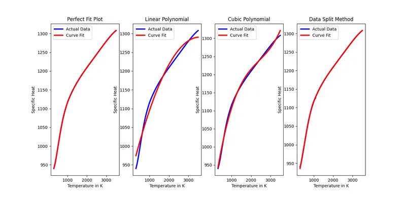
Linear fit – From the plots we can compare how far the points of curve fit are from the original data set and so we can say that error is large and hence cannot be called a perfect fit.

Cubic fit - From the plots we can compare the points of curve fit are still a bit far from the original data set but much closer to the curve obtained from linear polynomial model. Hence, we can say that by increasing the degree of polynomial we could get a better fit curve.

5. What needs to be done in order to make the curve fit perfectly?

There a multiple way to obtain a perfect fit for a given data sample.

By increasing the degree of polynomial, the error could be minimized to great extents and a perfect fit could be obtained. But the computational time increases as the degree of polynomials gets higher.

We can also apply split method where we can split the data at certain intervals and create unique coefficients for lower order polynomials and then finally add up all the data into one variable. Here we could use a lower order polynomial like cubic or linear to obtain a fit closer to perfect fit depending on the splits made.

6. Show empirically as to how well your curve has been fit.

By visuals we can see that plot 1 and plot 4 shows curve very close to the original model and hence we can conclude a perfect fit has been achieved.

#Python code for Curve_fit assignment
import matplotlib.pyplot as plt
import math
from scipy.optimize import curve_fit
import numpy as np
#Importing required modules to perform Curve Fit

#Defined three different functions to perform curve fit with linear polynomial,cubic polynomial and with 10 polynomials
def func(t,a,b,c,d,e,f,g,h,i,j,k):
	return(pow(t,10)*a+pow(t,9)*b+pow(t,8)*c+pow(t,7)*d+pow(t,6)*e+pow(t,5)*f+pow(t,4)*g+pow(t,3)*h+pow(t,2)*i+t*j+k)
def linear(t,a,b,c):
	return(pow(t,2)*a+t*b+c)
def cubic(t,a,b,c,d):
	return(pow(t,3)*a+pow(t,2)*b+t*c+d)

#Function to read the text file and extract values from every line
def read_file():
	temperature=[]
	cp=[]
	for line in open('data','r'):
		#Since the data file is arranged in such a manner that temperature and cp 
		#are set apart by means of a ',' we can use line.split command
		value = line.split(',')
		temperature.append(float(value[0]))
		cp.append(float(value[1]))
	return [temperature,cp]

#Calling the function and storing the values of temperature and cp in variables
#For 10 polynomials curve fit
temperature,cp=read_file()
popt,pcov =curve_fit(func,temperature,cp)
#For the polynomials extracted from the curve_fit function a new cp data can be created and plotted to check how it follows
#the trend and how close the values are to the original plot
fit_cp = func(np.array(temperature),*popt)
#For linear polynomials curve fit
popt,pcov =curve_fit(linear,temperature,cp)
fit_cp2 = linear(np.array(temperature),*popt)
#For cubic polynomials curve fit
popt,pcov =curve_fit(cubic,temperature,cp)
fit_cp3 = cubic(np.array(temperature),*popt)

#Trying Data Split method by splitting the whole data into 4 equal lengths parameter 
ran = int(len(temperature)/4)
temperature1 = temperature[0:ran]
temperature2 = temperature[ran:(ran*2)]
temperature3 = temperature[(ran*2):(ran*3)]
temperature4 = temperature[(ran*3):(ran*4)]
cp1 = cp[0:ran]
cp2 = cp[ran:(ran*2)]
cp3 = cp[(ran*2):(ran*3)]
cp4 = cp[(ran*3):(ran*4)]
#Every Temperature and Cp variable carries a total of 800 values 
#For every individual data a cubic polynomial with unique coefficients would be created 
for j in range(0,ran):
	popt,pcov =curve_fit(cubic,temperature1,cp1)
	fit_cp41=cubic(np.array(temperature1),*popt)
for j in range(ran,(ran*2)):
	popt,pcov =curve_fit(cubic,temperature2,cp2)
	fit_cp42=cubic(np.array(temperature2),*popt)
for j in range((ran*2),(ran*3)):
	popt,pcov =curve_fit(cubic,temperature3,cp3)
	fit_cp43=cubic(np.array(temperature3),*popt)
for j in range((ran*3),(ran*4)):
	popt,pcov =curve_fit(cubic,temperature4,cp4)
	fit_cp44=cubic(np.array(temperature4),*popt)

#Once all the values for fit_cp curve is generated we can store all into a single variable and plot it 
fit_cp4 = []
for val in fit_cp41:
	fit_cp4.append(val)
for val in fit_cp42:
	fit_cp4.append(val)
for val in fit_cp43:
	fit_cp4.append(val)
for val in fit_cp44:
	fit_cp4.append(val)

#Plotting every plots seperately using Subplot command to display all in the same figure
plt.subplot(1,4,1)
plt.plot(temperature,cp,color='blue',linewidth=3)
plt.plot(temperature,fit_cp,color='red',linewidth=3)
plt.legend(['Actual Data','Curve Fit'])
plt.xlabel('Temperature in K')
plt.ylabel('Specific Heat')
plt.title('Perfect Fit Plot')
plt.subplot(1,4,2)
plt.plot(temperature,cp,color='blue',linewidth=3)
plt.plot(temperature,fit_cp2,color='red',linewidth=3)
plt.legend(['Actual Data','Curve Fit'])
plt.xlabel('Temperature in K')
plt.ylabel('Specific Heat')
plt.title('Linear Polynomial')
plt.subplot(1,4,3)
plt.plot(temperature,cp,color='blue',linewidth=3)
plt.plot(temperature,fit_cp3,color='red',linewidth=3)
plt.legend(['Actual Data','Curve Fit'])
plt.xlabel('Temperature in K')
plt.ylabel('Specific Heat')
plt.title('Cubic Polynomial')
plt.subplot(1,4,4)
plt.plot(temperature,cp,color='blue',linewidth=3)
plt.plot(temperature,fit_cp4,color='red',linewidth=3)
plt.legend(['Actual Data','Curve Fit'])
plt.xlabel('Temperature in K')
plt.ylabel('Specific Heat')
plt.title('Data Split Method')
plt.show()

Conclusion:

The Python code has been designed such that it would plots results for a linear curve fit, cubic curve fit, high order polynomial fit and curve fit using split method.