Week 2 Air standard Cycle

Aim:

To Simulate generic code for Otto Cycle in Python

Governing Equations:

An Otto cycle is an idealized thermodynamic cycle that describes the functioning of a typical spark ignition piston engine.

The Otto Cycle, describes how heat engines turn gasoline into motion. Like other thermodynamic cycles, this cycle turns chemical energy into thermal energy and then into motion. The Otto cycle describes how internal combustion engines (that use gasoline) work, like automobiles and lawn mowers.

Objective:

To simulate generic code for Otto Cycle and calculate its thermal efficiency.

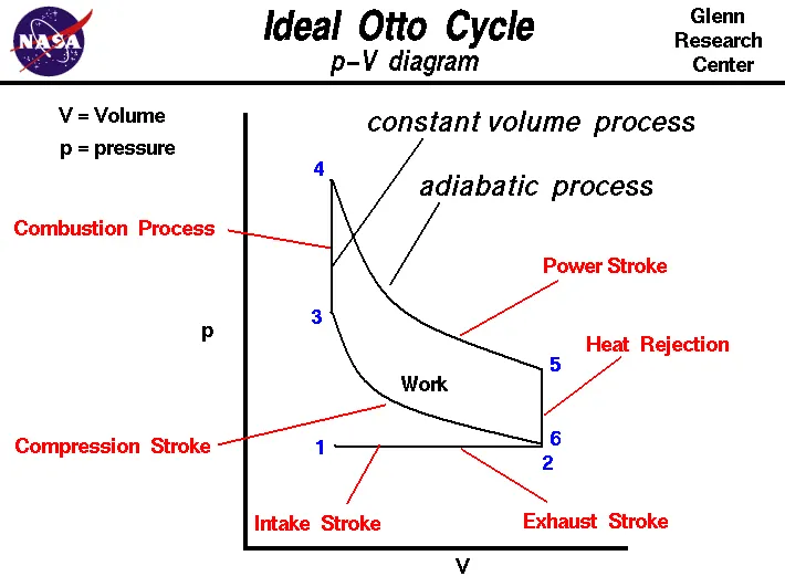
Process 2-3 – Compression Stroke – Isentropic Thermal Compression takes place. Where

PV^gamma = Constant

Process 3-4 – Combustion Process – Constant Volume Heat addition process. Following Ideal gas law

PiVi/Ti = PjVj/Tj

Process 4-5 – Power Stroke – Isentropic Thermal Expansion takes place. Where

PV^gamma = Constant

Process 5-6 – Exhaust Stroke – Constant Volume Heat Rejection process. Following Ideal gas law

PiVi/Ti = PjVj/Tj

#Python Code to generate Otto Cycle P-V Plot and calculate thermal efficiency of the engine.

import math
import matplotlib.pyplot as plt
import numpy as np

#Function to get volume at different crank angles

def engine_kinematics(bore,stroke,con_rod,cr,start_crank,end_crank):

	#Engine Parameters Calculations
	#Crank pin radius and ratio of connecting rod lenght and crank pin radius
	a=stroke/2
	r = con_rod/a

	#Volume Calculations
	v_s = (math.pi/4)*pow(bore,2)*stroke
	v_c = v_s/(cr-1)

	#Initialing a variable num_val to capture trend of P-V during Isentropic process 
	num_val = 50
	#Converting theta values input into radians
	sc = math.radians(start_crank)
	ec = math.radians(end_crank)
	#Dividing equal halfs for values between starting crank angle and end crank angle excluding the value of end crank angle
	dtheta = (ec-sc)/(num_val-1)
	#Creating an empty volume array to store values for Volume based on the formula

	V = []

	for i in range (0,num_val):
		#V/v_c=1+0.5(cr-1)[R+1-cos(theta)-(r^2-sin^2(theta)^0.5)]
		#Dividing the above formula into three terms to simplify the code
		theta = sc+(dtheta*i)
		term1 = 0.5*(cr-1)
		term2 = r+1-math.cos(theta)
		term3 = pow(pow(r,2)-pow(math.sin(theta),2),0.5)
		#Storing every value in the empty array
		V.append(v_c*(1+(term1*(term2-term3))))
	#Returning the value of V when the function would be called
	return V

# Inputs
p1 = 101325 #Pascals equal to 1 atm - Inlet Mixture Pressure
t1= 500 #K - Inlet Mixture Temperature
t3 = 2300 #K - Combustion Temperature
gamma = 1.4

#Engine Parameters input
bore = 0.1
stroke = 0.1
con_rod = 0.15
cr = 12

#Volume Calculations
v_s = (math.pi/4)*pow(bore,2)*stroke
v_c = v_s/(cr-1)

#State 1 Variable
#Mixture enters the Combustion Chamber
#Since the Piston is on the BDC volume to be covered will be equal to Swept volume + compression Volume
v1= v_s+v_c

#State 2 Variables
#Now after the mixture has been compressed and the piston is at TDC
v2= v_c
#In between State 1 and 2 an Isentropic process takes place
#Calling the function and storing the values in variable V
V_compression = engine_kinematics(bore,stroke,con_rod,cr,0,180)
#Since we know PV^gamma is a constant so extracting the constant value from State point 1 and then using the value to find 
#values for Pressure for every value of volume
constant = p1*pow(v1,gamma)
P_compression = []
for v in V_compression:
	#For every element in V_compression array we are calculating value of pressure and storing it in another array
	P_compression.append(constant/(pow(v,gamma)))

#Following Isentropic Expansion [p1v1^gamma = p2v2^gamma]
p2 = (p1*pow(v1,gamma))/(pow(v2,gamma))
#Following Ideal gas law [p2v2/t2 = p1v1/t1]
t2 = t1*(p2*v2)/(p1*v1)

#State 3 Variables
#Constant Volume heat addition would take place in the power stroke therefore v3=v2
v3=v2
#Again following Ideal gas law to extract p3 [p3v3/t3 = p2v2/t2]
p3 = ((p2*v2*t3)/(t2*v3))
#Similar to what we did for Compression process
constant = p3*pow(v3,gamma)
V_expansion = engine_kinematics(bore,stroke,con_rod,cr,180,0)
P_expansion = []
for v in V_expansion:
	P_expansion.append(constant/(pow(v,gamma)))

#State 4 Variables
#Since it would be an exhaust stroke piston would be at BDC and hence v4 would be equal to v1
v4 = v1
#Following Isentropic Compression [p4v4^gamma = p3v3^gamma]
p4 = (p3*pow(v3,gamma))/pow(v4,gamma)
#Again following Ideal gas law to extract p3 [p4v4/t4 = p3v3/t3]
t4 = t3*(p4*v4)/(p3*v3)

#Thermal Efficiency = 1- (1/(cr^(gamma-1))
eff = (1-(1/(pow(cr,(gamma-1)))))*100
print('Efficiency of Otto Cycle is ',eff,'%')

#Plots for state points
#By mentioning the color within the plot statement all the lines would be displayed in the same color
plt.plot([v2,v3],[p2,p3],color='red')
plt.plot(V_expansion,P_expansion,color='red')
plt.plot(V_compression,P_compression,color='red')
plt.plot([v4,v1],[p4,p1],color='red')
#Using text keyword to print the State points for better understanding
plt.text((v1+0.00001),(p1-200000),str('1'),color='blue')
plt.text((v2-0.00002),(p2-200000),str('2'),color='blue')
plt.text((v3+0.00002),(p3+50000),str('3'),color='blue')
plt.text((v4+0.00001),(p4+200000),str('4'),color='blue')
plt.xlabel('Volume (m^3)')
plt.ylabel('Pressure (Pa)')
plt.title('Otto Cycle')
plt.show()

Conclusion:

The Python code has been designed such that the values for engine parameters like bore, stroke, compression ratio, start crank angle, end crank angle can be given as input and P-V Plot can be obtained for the same.

Also, thermal efficiency of the cycle is printed.