Week 5 - Curve fitting

Curve fitting

What do popt and pcov mean?

popt- It helps to minimize the sum of the squared error of function data by an array of optimal values of parameters

pcov- The estimated covariance of popt or in other words tells that how far the variables may change together. The diagonals provide the variance of the parameter estimate.

What does np.array(temperature) do?

The temperature values will be taken and pass as a numpy array to perform certain mathematical operations.

What does the * in *popt mean?

This is used to tell that this is stored in a popt array. It contains the value of coefficients and refers to these values.

Main Code:

• In the main programme, we call the function using read_file that contained specific heat of o2 as a function of temperature.
• When we execute the data file the values will be stored in temperature and cp value.
• For that, we define a linear and cubic function.
• We initialise the empty array for cp and temperature.
• Now in for loop, we open a file data with 'r' means in reading mode line by line.
• Separate the data with ','.
• 1st is the temperature value and the second is the cp.
• As they are in a text file as a string so we have to convert them using 'float' to use in the calculation.
• Append them and return to cp.
• Now we use the curve_fit function in the scipy module with its parameters.
• The first input is the mathematical model that is using to represent our data. The function is in this case linear and cubic.
• With this, we get 1 output- popt (they are the coefficients a,b in linear function) and pcov.
• Once we have new coefficients we take the function that we defined and pass the temperature array along with the coefficients.
• With curve fit, we calculate the cp again, that called fit_cp and plot them.

For linear Equation

import math
import numpy as np
import matplotlib.pyplot as plt
from scipy.optimize import curve_fit

def linear(t, a, b):    # Linear curve fit function
	return a*t + b

def read_file():
	temperature = []
	cp = []
	for line in open('data','r'):
		values=line.split(',')
		temperature.append(float(values[0]))
		cp.append(float(values[1]))
	return [temperature, cp]

#Main programe

temperature, cp = read_file()    # Reading original values of data
popt,pcov = curve_fit(linear, temperature, cp)
fit_cp = linear(np.array(temperature), *popt)

# Plot

plt.plot(temperature, cp,,linewidth=3)
plt.plot(temperature, fit_cp,,linewidth=3)
plt.legend(['Actual data', 'curve fit data'])
plt.xlabel('Temperature [k]')
plt.ylabel('cp')
plt.show()

For cubic Equation

import math
import numpy as np
import matplotlib.pyplot as plt
from scipy.optimize import curve_fit

def func(t,a,b,c,d):
	return a*pow(t,3)+ b*pow(t,2) + c*t + d


def read_file():
	temperature = []
	cp = []
	for line in open('data','r'):
		values=line.split(',')
		temperature.append(float(values[0]))
		cp.append(float(values[1]))
	return [temperature, cp]

#Main programe

temperature, cp = read_file()    # Reading original values of data
popt,pcov = curve_fit(func, temperature, cp)
fit_cp = func(np.array(temperature), *popt)

# Plot

plt.plot(temperature, cp,,linewidth=3)
plt.plot(temperature, fit_cp,,linewidth=3)
plt.legend(['Actual data', 'curve fit data'])
plt.xlabel('Temperature [k]')
plt.ylabel('cp')
plt.show()

Results:

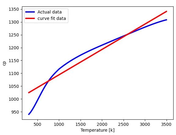
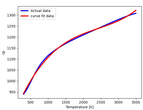
From both these above linear and cubic curve fit it can be easily seen that if we increase the order of polynomial the both the observed and curve fit data curve will be closer that means we will have better results with the cubic fit.

In this way we can improve the result of our curve fit with higher-order polynomial, however, it can not be completely free from error.