Week 5 - Curve fitting

Objective: To write a code to find a linear and cubic polynomial curve fit with the given Cp data and show empirically how well it fits with the data.

Introduction:

Curve fitting is the process of constructing a curve, or mathematical function, which possesses closest proximity to the real series of data. By curve fitting, we can mathematically construct the functional relationship between the observed dataset and parameter values.

1.popt- It is an argument used to find the values of the parameters a and b.

pcov -the covariance of the array of parameters in popt and helps in finding the deviation errors in popt.

2. np.array(temperature) - it stores the values of the temperature in the form of array and sends it to numpy function.

3.*in*popt - it means it stores the values of the constant parameters a,b,c in popt .

Code for linear and cubic curve fit:

import numpy as np 
import matplotlib.pyplot as plt 
from scipy.optimize import curve_fit 
# linear curve fit 
def func_linear(t,a,b):
	return a*t+b
#reading the data
def read_file():
	temperature=[]
	cp=[]
	for line in open('data','r'):
		values=line.split(',')
		temperature.append(float(values[0]))
		cp.append(float(values[1]))
	return[temperature,cp]
	
temperature,cp=read_file()
popt,pcov=curve_fit(func_linear,temperature,cp)
fit_cp=func_linear(np.array(temperature),*popt)
plt.plot(temperature,cp,color="blue",linewidth=3)
plt.plot(temperature,fit_cp,color="red",linewidth=3)
plt.title('specific heat vs temperature')
plt.xlabel('temperature[k]')	
plt.ylabel('cp')
plt.show()

# cubic curve fit 
def func_linear(t,a,b,c,d):
	return a*pow(t,3)+b*pow(t,2)+c*t+d
#reading the data
def read_file():
	temperature=[]
	cp=[]
	for line in open('data','r'):
		values=line.split(',')
		temperature.append(float(values[0]))
		cp.append(float(values[1]))
	return[temperature,cp]
	
temperature,cp=read_file()
popt,pcov=curve_fit(func_cubic,temperature,cp)
fit_cp=func_cubic(np.array(temperature),*popt)
plt.plot(temperature,cp,color="blue",linewidth=3)
plt.plot(temperature,fit_cp,color="red",linewidth=3)
plt.title('specific heat vs temperature')
plt.xlabel('temperature[k]')	
plt.ylabel('cp')
plt.show()

Plot for linear curve fit: Plot for the cubic polynomial:

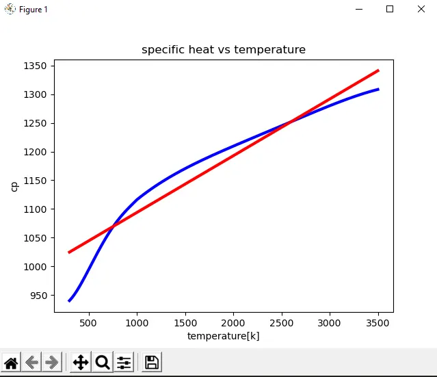
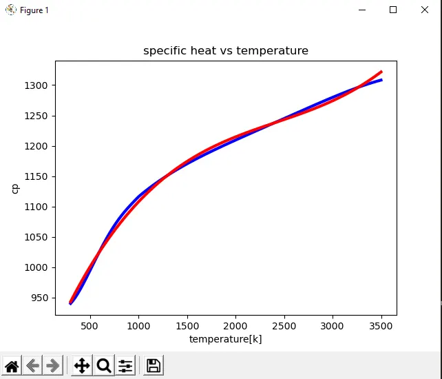
From the above plots its clearly seen that linear polynomial has greater deviations and doesn't match exactly with the given data,whereas the cubic polynomial has close to exact match with the given data.There are only minor deviations in the values for cubic polynomial.

Results: Hence the higher order polynomial makes exact match with given data than the lower order polynomial.