Week 2 Air standard Cycle

Aim: To simulate the Otto cycle using Python.

Theory:

An Otto cycle is a thermodynamic cycle that describes the functioning of a typical spark ignition piston engine. It is  most commonly found in automobile engines.

The Otto cycle is constructed from:

• Top and bottom of the loop: isentropic process(frictionless, adiabatic reversible).
• Left and right sides of the loop: an isochoric process (constant volume).

The processes are described by:

• Process 0–1 a mass of air is drawn into piston/cylinder arrangement at constant pressure.
• Process 1–2 is an adiabatic (isentropic) compression of the charge as the piston moves from bottom dead center (BDC) to top dead center (TDC).
• Process 2–3 is a constant-volume heat transfer to the working gas from an external source while the piston is at top dead center. This process is intended to represent the ignition of the fuel-air mixture and the subsequent rapid burning.
• Process 3–4 is an adiabatic (isentropic) expansion (power stroke).
• Process 4–1 completes the cycle by a constant-volume process in which heat is rejected from the air while the piston is at bottom dead center.
• Process 1–0 the mass of air is released to the atmosphere in a constant pressure process.

"""
otto cycle simulator
"""
import math
import matplotlib.pyplot as plt
#defining variables
def engine_kinematics(bore,stroke,con_rod,cr,start_crank,end_crank):
#inputs
	a = stroke/2
	R = con_rod/a
#volume parameters
	#swept volume
	V_s=math.pi*(1/4)*pow(bore,2)*stroke
	#clearance volume
	V_c=V_s/(cr-1)
	#start and end points of crank 
	sc=math.radians(start_crank)
	ec=math.radians(end_crank)
	num_values=50
	dtheta=(ec-sc)/(num_values-1)
	V=[]
	for i in range(0,num_values):
		theta=sc+i*dtheta
		term1= 0.5*(cr-1)
		term2= R+1-math.cos(theta)
		term3=pow(R,2)-pow(math.sin(theta),2)
		term3=pow(term3,0.5)
		V.append((1+term1*(term2-term3))*V_c)
	return V
   
#inputs
#pressure at state1
p1=101325
#temperature at state 1
t1=500
gamma=1.4
#temperature at state 3
t3=2300
#parameters
bore=0.1
stroke=0.1
con_rod=0.15
cr=5
#volume calculation
#state 1
V_s=(math.pi/4)*pow(bore,2)*stroke
V_c=V_s/(cr-1)
V1=V_c+V_s
#state 2 
V2=V_c
#p2v2^gamma=p1v1^gamma
p2=p1*pow(V1,gamma)/pow(V2,gamma)
#p2v2/t2=p1v1/t1|rhs=p1v1/t1|p2v2/t2=rhs|t2=p2v2/rhs
rhs=p1*V1/t1 
t2=p2*V2/rhs
V_compression=engine_kinematics(bore,stroke,con_rod,cr,180,0)
constant=p1*pow(V1,gamma)
P_compression=[]
for V in V_compression:
	P_compression.append(constant/pow(V,gamma))
#state 3
V3=V2
#p3v3/t3=p2v2/t2|rhs=p2v2/t2|p3=rhs*t3/v3
rhs=p2*V2/t2
p3=rhs*t3/V3
V_expansion=engine_kinematics(bore,stroke,con_rod,cr,0,180)
constant=p3*pow(V3,gamma)
P_expansion=[]
for V in V_expansion:
	P_expansion.append(constant/pow(V,gamma))
#state 4
V4=V1
#p4v4^gamma=p3v3^gamma
p4=p3*pow(V3,gamma)/pow(V4,gamma)
#p4v4/t4=rhs
t4=p4*V4/rhs
#thermal efficiency calculation
eff=(1-((t4-t1)/(t3-t2)))*100
print(eff)
#plotting 
plt.plot([V2,V3],[p2,p3])
plt.plot(V_compression,P_compression)
plt.plot(V_expansion,P_expansion)
plt.plot([V4,V1],[p4,p1])
plt.xlabel('Volume')
plt.ylabel('Pressure')
plt.title('Otto cycle')
plt.show()

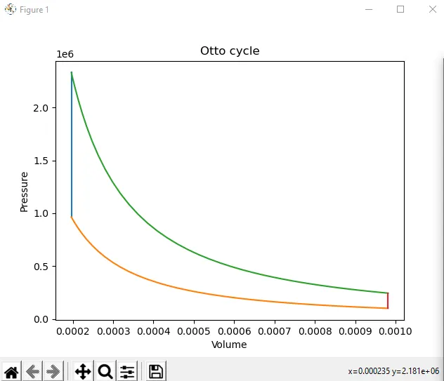
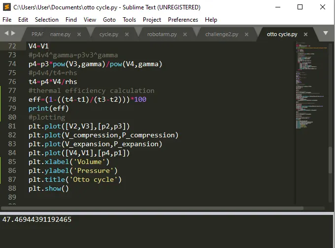
Output:

Hence the PV diagram and the thermal efficiency were calculated using the python code.