Week 5 - Curve fitting

Q1 What does popt and pcov mean?

popt- An array of optimal Values for the parameters which minimize the sum of squares of residuals.

pcov- 2d array which contains the estimated covariance of popt.The diagonals provide the variance of the parameter estimate.

Q2 What does np.arry(temperature) do?

np.array-converts the python list of temperature to a numpy array since operations like pow are allowed on numpy array and not python lists.

Q3 What does the *in* popt mean?

*-reference to opt/the values stored in the array popt.

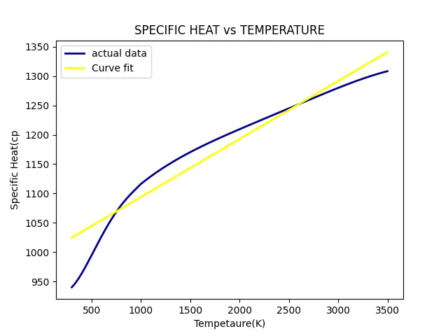
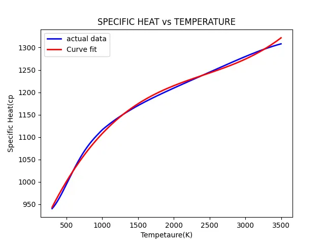
Q5 What needs to be done in order to make the curve fit perfect?

• By Increasing the degree of the curve we can make the best curve fit.
• If we further increase the degree of the curve to 4 then the curve will be more accurate than the cubic polynomial.
• Furthur Increasing the degree of the polynomial will increase the calculated complexity and time required, hence 4th order polynomial can be taken as a sufficient curve fit.

# Importing the modules
import numpy as np 
import matplotlib.pyplot as plt
from scipy.optimize import curve_fit
#defining Linear function
def func1(t,a,b):
	return a*t+b 
	# a,b are constants
# Defining function to read dats
def read_file():
	tempetaure=[]
	cp=[]
	for line in open('data','r'):
		values=line.split(',')
		tempetaure.append(float(values[0]))
		cp.append(float(values[1]))
	return [tempetaure,cp]
#Main Function
tempetaure,cp=read_file()
popt,pcov=curve_fit(func1,tempetaure,cp)
fit_cp=func1(np.array(tempetaure),*popt)
# Plottinf for Linear Curve
plt.figure('1')
plt.plot(tempetaure,cp,color='Darkblue',linewidth=2)
plt.plot(tempetaure,fit_cp,color='yellow',linewidth=2)
plt.title('SPECIFIC HEAT vs TEMPERATURE')
plt.legend(['actual data','Curve fit'])
plt.xlabel('Tempetaure(K)')
plt.ylabel('Specific Heat(cp')
plt.savefig('Linear')
plt.show()
#Defining Cubic polynomial
def func2(t,a,b,c,d):
	return a*pow(t,3)+b*pow(t,2)+c*t+d
	# a,b,c,d are constants
tempetaure,cp=read_file()
popt,pcov=curve_fit(func2,tempetaure,cp)
fit_cp=func2(np.array(tempetaure),*popt)
#plotting for cubic polynomial
plt.figure('2')
plt.plot(tempetaure,cp,color='blue',linewidth=2)
plt.plot(tempetaure,fit_cp,color='red',linewidth=2)
plt.title('SPECIFIC HEAT vs TEMPERATURE')
plt.legend(['actual data','Curve fit'])
plt.xlabel('Tempetaure(K)')
plt.ylabel('Specific Heat(cp')
plt.savefig('Cubic polynomial')
plt.show()

code explanation:

1. The first step in developing this code is importing the modules.

2. The next step is defining a linear function.

a*t+b, Where a,b are constants

and t is temperature

3. The next step is defining read_file(): function in order to read the data from the data file.

4. tempetaure=[]
cp=[]

Created two arrays to store the temperature and cp values.

5. By using the for loop we stored all temperature and cp values in respective arrays.

6. Next used the popt and pcov in order to find covariance and for the constants.

7. Next by using fit_curve function we fit a curve.

8.Then drawn the plots for temperature vs cp and temperature vs fit_cp.

9. Then again created a function for cubic polynomial.

10. Then again used the popt and pcov in order to find covariance and for the constants.

11 Next, by using fit_curve function we fit a curve.

12.Then drawn the plots for temperature vs cp and temperature vs fit_cp.

13.The outputs are stored and attached here.