Week 5 - Curve fitting

1) "popt" gives the optimum values from the equation i.e,the coefficients of the polynomial. "pcov" gives the covariance of the polynomial.

2)The Numpy library used as "np" is used to perform various functions with a list. In here Temperature is a list and np command helps in multiplying it with the coefficients.

3) The "*" in *popt is used to multiply a single integer with a list.

4) Aim:

To perform Curve fit of a linear and Cubic polynomial using Python.

Theory:

Curve Fit:

Curve fitting is the reffered to the process of creating a mathematical function or constructing a curve that has the closest proximity to the original data.Curve fitting is used to construct a mathematical function which relates to the inputs to the data,which could predict the dataset.This predicted data set may not be exactly the same as it works on the proximity.The higher the order of the polynomial the better is the curve fit.There are four parameters that define the goodness of the curve fit.They are,

1. Sum of Squares due to errors (SSE)
2. R square(R)
3. Adjusted R square
4. Root means Squared errors(RMSE)

The higher the value of R ,the better is the curve.R=0 is the worst possible fit for the dataset where as R=1 is the best possible fit.R>0.95 is considered as a good fit to the curve.

Despcription of Program:

• Program 1:

1. The data set is called into the program and the initial conditions are set.
2. 2 Functions are written for linear and cbic polynomial and are called in the program when required.
3. Data is extracted from the file as temperature and Cp.
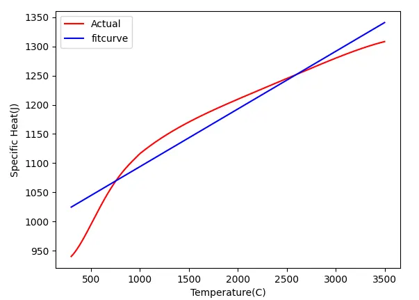
4. Using the "curve_fit" command the data are assigned to a linear polynomial equation.
5. The curve_fit command gives the optimal values i.e, the coefficients and covariance.
6. Using the "plot" command both the actual Cp and the predicted Cp are plotted
7. This gives a curve fit.
8. Similarly,step 2-4 are repeated to assign a cubic polynomial and a correspomding fit is obtained.

import math
import matplotlib.pyplot as plt
import numpy as np 
from scipy.optimize import curve_fit

def func1(t,a,b):
	return a*t + b

def func2(t,c,d,e,f):
	return c*pow(t,3) - d*pow(t,2) + e*t -f


def read_file():
	temp = []
	cp = []
	f = open('data','r')
	for line in f:
		values = line.split(',')
		temp.append(float(values[0]))
		cp.append(float(values[1]))
	return [temp,cp]


temp,cp = read_file()
#print(temp,cp)

popt,pcov = curve_fit(func1,temp,cp)
fit = func2(np.array(temp), *popt)
plt.plot(temp,cp,color = 'red')
plt.plot(temp,fit,color = 'blue')
plt.xlabel('Temperature(C)')
plt.ylabel('Specific Heat(J)')
plt.legend(['Actual','fitcurve'])
plt.show()

Linear Polynomial Output:

Cubic Polynomial Output:

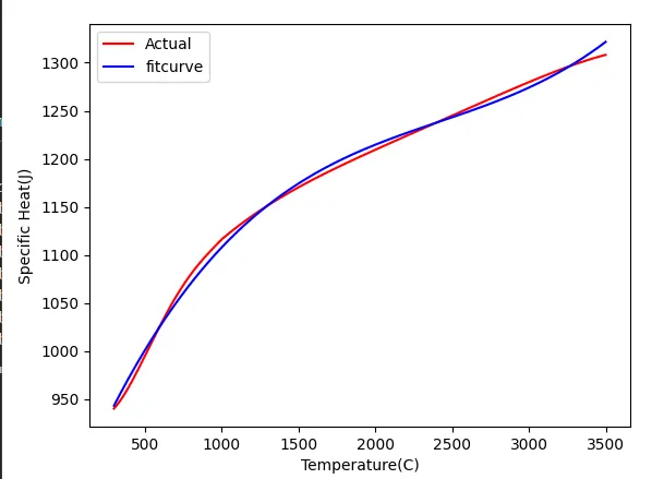
5) The higher the order of polynomial, the better is the fit.