Aim: Python programming for Curve Fit.

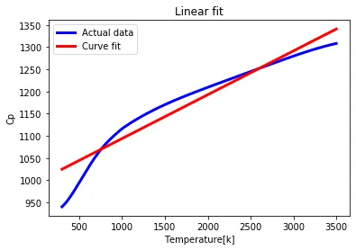
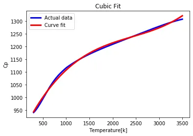
Objective : Write a code to fit a linear and cubic polynomial for the Cp data.

Theory: Curve fitting is the process of constructing the curve or mathematical function that has the best fit to a series of data points, possibly subjected to constraints. Curve fitting can involve either interpolation where an exact fit to the data is required or smoothing in which a smooth function is constructed that approximately fits the data. A related topic is regression analysis which focusses more on questions of statistical inference such as how much uncertainty is present in a curve that is fit to data observed with random errors.
Most commonly , one fits a function of the form y = f(x).
The first degree polynomial equation
y = a*x + b
is a line with a slope a. A line will connect any two points, so a first degree polynomial equation is an exact fit through any two points with distinct x coordinates.
If the order of the equation is increased to a second degree polynomial, the following results:
y = a*x2 + b*x + c
This will exactly fit the curve to three points.
If the order of the equation is increased to a third degree polynomial, the following is obtained:
y = a*x3 + b*x2 +c*x + d
This will exactly fit four points.

1)	What does popt and pcov mean?
Ans: popt means the coefficient of the polynomials. For eg a,b,c,d are the coefficients. Pcov refers to the covariance matrix for the estimated factors.
2)	What does np.array(temperature) do.
Ans: It creates the array of the temperature values from data file into a matrix.
3)	What does the *in* popt mean?
Ans: popt contains to the values of coefficient. The *in* helps us refer the values for these coefficients.
4)	What needs to be done in order to make the curve fit?
Ans: We need to increase the order of the polynomial to make the curve fit.

Python Code:
"""
Python code to fit a linear and cubic polynomial for the Cp data
"""

import numpy as np
import matplotlib.pyplot as plt
from scipy.optimize import curve_fit

# Curve fit function

def func(t,a,b):
    return a*t + b

def func_1(t,a,b,c,d):
    return a*pow(t,3)+b*pow(t,2)+c*t+d

# Reading thermodynamic data file

def read_file():
    temperature = []
    cp = []
    for line in open('data','r'):
        values = line.split(',')
        temperature.append(float(values[0]))
        cp.append(float(values[1]))

    return [temperature, cp]

# Main program for linear fit
temperature, cp = read_file()
popt, pcov = curve_fit(func,temperature,cp)
fit_cp = func(np.array(temperature),*popt)

plt.figure(1)
plt.plot(temperature, cp,,linewidth ="3")
plt.plot(temperature,fit_cp, color ="red", linewidth = "3")
plt.legend(['Actual data','Curve fit'])
plt.xlabel('Temperature[k]')
plt.ylabel('Cp')

# Main program for cubic fit

popt, pcov = curve_fit(func_1,temperature,cp)
fit_cp_1 = func_1(np.array(temperature),*popt)

plt.figure(2)
plt.plot(temperature, cp,,linewidth ="3")
plt.plot(temperature,fit_cp_1, color ="red", linewidth = "3")
plt.legend(['Actual data','Curve fit'])
plt.xlabel('Temperature[k]')
plt.ylabel('Cp')

Explanation of the code:
1)	Numpy, Matplolib libraries are imported. To import curve fit function, scipy.optimize function is used.
2)	To fit the linear and cubic curve, linear and cubic polynomial functions are used. Function(func) is used for linear polynomial while Function(func_1) is used for cubic polynomial.
3)	To read the data file for temperature and cp, the function read_file is defined. For loop is used to open the data file, split command is used to split the temperature and cp values using ‘,’. Finally the temperature command is used to append the temperature and cp values into the arrays.
4)	Main program for linear fit and cubic fit are written. Curve_fit function is used to calculate popt and pocv. Further the calculated values are stored by calling func and func_1 functions for linear and cubic equations and stored in fit_cp and fit_cp1 functions.
5)	The plot of fit_cp and and actual values are plotted for linear and cubic equation.

Conclusion: As we can see  from the graph that for a cubic fit, the curve fit passes through maximum data points as compared to linear fit. Hence we can infer that increasing the degree of polynomial makes the curve best fit.