Week 5 - Curve fitting

Week 5 Challenge - Curve Fitting

1. What does popt and pcov mean? (Watch the video to get some context)

2. What does np.array(temperature) do?

3. What does the * in *popt mean?

4. Write code to fit a linear and cubic polynomial for the Cp data. Explain if your results are good or bad.

5. What needs to be done in order to make the curve fit perfect?

6. Show empirically as to how well your curve has been fit.

ANS 1:

In the curve fitting code, the variables "popt" and "pcov" are defined to the curve fit function. The first variable, "popt", stores and extracts the coefficients of the curve fitting function into an array, with respect to the general polynomial equation defined in the curve fit function. In this assignment, there are two curve fit functions used for a linear and cubic model. For each mode, the "popt" variable will be an array with the coefficients of the linear and cubic model. The second variable, "pcov", represents a matrix in square form, which stores the covariance values of the coefficients stored in the array defined by the "popt" variable. The diagonal elements of this square matrix will match with the variance of the same coefficients.

ANS 2:

The "np.array(temperature)" command creates an array from the temperature values that were retrieved from the thermodynamic data file, using the "numpy" library. Having the temperature data in an array is useful in this code as it helps the code to calculate fitted "Cp" values for each respective temperature value based on the "popt" array.

ANS 3:

The "*" in the "*popt* tells the python code to indicate and return the values of the coefficients that are stored in the "popt" array.

ANS 4:

The python code for the linear curve fit model is shown in the section of code below:

import numpy as np 
import matplotlib.pyplot as plt 
from scipy.optimize import curve_fit


# Linear Fit Function
def linear_func(t, a, b):
	return a*t + b


# Reading Thermodynamic File
def read_file():
	temperature = []
	cp = []
	for line in open('data', 'r'):
		values = line.split(',')
		temperature.append(float(values[0]))
		cp.append(float(values[1]))

	return [temperature, cp]


# Main Program
temperature, cp = read_file()

# Linear Curve Fitting
popt, pcov = curve_fit(linear_func, temperature, cp)
fit_cp1 = linear_func(np.array(temperature), *popt)
plt.plot(temperature, cp, color = "blue", linewidth = 3)
plt.plot(temperature, fit_cp1, color = "red", linewidth = 3)
plt.legend(["Actual Data", "Curve Fit"])
plt.xlabel("Temperature [K]")
plt.ylabel("Cp")
plt.show()


total_cp = np.sum(cp)
numval_cp = np.size(cp)
avg_cp = total_cp/numval_cp
print('Average Cp is:', avg_cp)

# GOF Characteristics

for i in range(numval_cp):
	sst = np.sum(pow((cp[i]-avg_cp),2))
	ssr = np.sum(pow((cp[i]-fit_cp1[i]),2))

# R-Squared Value
r_squared = 1-(ssr/sst) 
print("R-Squared:", r_squared)

# Root Mean Square Error (RMSE)
rmse = pow((ssr/numval_cp),0.5)
print("RMSE:", rmse)

First, the basic python libraries of "numpy", "matplotlib.pyplot" are imported into the python script along with the "curve_fit" function from the "scipy" module. Next, a function is created with the basic structure of the linear model with the variables of a, t, and b. The linear model will be of the form, `y = mx+c`i.e. a straight line.

Next, another function called "read_file" is created to read the thermodynamic file data. Within this function, two empty arrays are created for the temperature and "Cp" data. After this, a for loop is created that reads the data from the thermodynamic file by specifying the file name, "data" and the variable "r" which represents reading the data from the "data" file. This command will only be successful if the data file is located in the same directory as the python script. Within the for loop, a variable called " values" is created to separate the temperature and "Cp" data from the thermodynamic data file wherever a comma is located in every line, using the "line.split" command. Finally, the for loop ends by adding the separated temperature and "Cp" data in to the respective empty arrays using the "append" command. The distinction is made between the temperature and "Cp" values using the index positions of 0 and 1 respectively. The function ends by returning the temperature and "Cp" values.

Then, the main program begins wherein the "read_file" function is called to retrieve the temperature and "Cp" data. Next, the curve fitting is performed using the "curve_fit" function from the "scipy" module. The variables of "popt" and "pcov" are created to store the values of the coefficients and the covriance of the coefficients respectively. Within the "curve_fit" function, the linear function named "linear_func" is called out along with the temperature and "Cp" values.

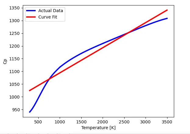
After this, a new variable, "fit_cp1" is created to store the fitted "Cp" values based on the linear model. This variable is defined by calling the "linear_func" function and storing the temperature values in to an array. The temperature values will have a corresponding fitted value for the "Cp" set of data using the "popt" variable. The plotting is performed for the two sets of data. The first set will contain the actual data from the thermodynamic file, whereas the second set will contain the fitted data. The plots are distinguished using different line colors and legends.

After the plotting, some statistical calculations were performed to determine the goodness of fit of the linear curve fit model. The goodness of fit is measured in a variety of methods, but in this case, I have measured the same using two parameters. The first is R-Squared value, and the second is the root mean squared error. To calculate either of these parameters, some prior calculations were performed.

First, the average or mean value for the "Cp" values in the thermodynamic data file was determined. This mean calculation was performed by first finding the total number of values for the "Cp" data and the sum of all of the "Cp" values using the "np.size" and "np.sum" commands from the "numpy" module.

For the goodness of fit calculations, a for loop was created. In this for loop, two terms were calculated. The first term is the total sum of squares. This term is calculated using the formula below:

`TSS = sum(y_i - bary) ^2`

where,

`y_i` - Original "Cp" value

`bary`- Average "Cp" value

Then, the second term was calculated called the sum of squares regression. This term is calculated using the formula below:

`SSR = sum(y_i - y_(fit)) ^2`

where,

`y_(fit)`- Fitted "Cp" value from the model

Finally, the R-Squared value and root mean squared error (RMSE) were calculated using the formulas shown below:

`R^2 = 1 - ((RSS)/(TSS))`

`RMSE = ((RSS)/n)^0.5`

where,

n - number of "Cp" values in the thermodynamic data file

The plot of the actual data with the fitted model is shown in the graph below:

The output results from the python code are shown below:

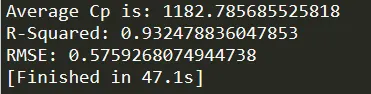
From this, we can see that the R-Squared value was 0.932 and the RMSE value was 0.576 to three decimal places. For the R-Squared value, the value must always lie between 0 and 1 for a valid measure. The closer the value is to 1, the better the goodness of fit for our model. The RMSE value can also take any value depending on the data set for which we are trying to perform the curve fit. However, the lower the RMSE value, the better the goodness of fit. In my case, the R-Squared value was considerably close to 1, and the RMSE value was considerably low. From these values, the fitted linear model was decent. However, from the graphical output, we can see that the linear model does not model the actual data very well.

The same process was followed for a cubic fitted model, shown in the section of code below:

import numpy as np 
import matplotlib.pyplot as plt 
from scipy.optimize import curve_fit


# Cubic Fit Function
def cubic_func(t, a, b, c, d):
	return a*pow(t,3) + b*pow(t,2) + c*t + d


# Reading Thermodynamic File
def read_file():
	temperature = []
	cp = []
	for line in open('data', 'r'):
		values = line.split(',')
		temperature.append(float(values[0]))
		cp.append(float(values[1]))

	return [temperature, cp]


# Cubic Curve Fitting
temperature, cp = read_file()
popt, pcov = curve_fit(cubic_func, temperature, cp)
fit_cp2 = cubic_func(np.array(temperature), *popt)
plt.plot(temperature, cp, color = "blue", linewidth = 3)
plt.plot(temperature, fit_cp2, color = "red", linewidth = 3)
plt.legend(["Actual Data", "Curve Fit"])
plt.xlabel("Temperature [K]")
plt.ylabel("Cp")
plt.show()

# GOF Characteristics
total_cp = np.sum(cp)
numval_cp = np.size(cp)
avg_cp = total_cp/numval_cp
print('Average Cp is:', avg_cp)

# Linear Curve GOF

for i in range(numval_cp):
	sst = np.sum(pow((cp[i]-avg_cp),2))
	ssr = np.sum(pow((cp[i]-fit_cp2[i]),2))

# R-Squared Value
r_squared = 1-(ssr/sst) 
print("R-Squared:", r_squared)


# Root Mean Square Error (RMSE)
rmse = pow((ssr/numval_cp),0.5)
print("RMSE:", rmse)

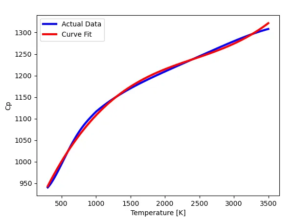
The output graph of this code is shown below:

The goodness of fit values from the code output are shown below:

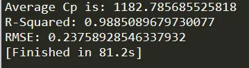
From the goodness of fit calculations, we can see that the R-Squared value was 0.989 and the RMSE value was 0.238 to three decimal places. Compared to the R-Squared value for the linear model, the cubic model was closer to a value of 1 and the RMSE value for the same was lower. From this perspective, the cubic model is a better fitted model than the linear model. From the graph output also, we can see that the cubic model follows the actual data set more closely. From these results, it is fair to say that the cubic model is far more superior to the linear model.

ANS 5:

To make the curve fit model better, there are two methods that can be followed. The first method involves adjusting the fitted function using a trial and error method and observing the changes in the graphical output to see if the model is a better fit to the actual data. There are unlimited combinations of coefficients to try and observe whether the model is a better fit or not. However, this method has a limitation with respect to the order of the polynomial. This is because no matter how many combinations of coefficients we try, the order of that model will only reach a maximum level of fit that cannot be exceeded. this is when the second method of using higher order polynomials is more useful. When using higher order polynomials, the fitted model will be a better fit to the actual data. This is because higher order polynomials have more coefficients and thus have more coefficients that can be adjusted to be a better fit. From the previous question, it was evident that the cubic fitted model was superior to the linear fitted model. The cubic fitted model had better goodness of fit characteristics and followed the shape of the actual data more closely on the graph.

ANS 6:

From the answer to question 4, the goodness of fit for the linear and cubic fitted models was explained based on the parameters of the R-Squared value and the RMSE. In addition, the graphical output for both models was also shown.