Week 5 - Curve fitting

Curve fitting

Introduction >

Curve fitting is a type of optimization that finds an optimal set of parameters for a defined function that best fits a given set of observations.

Following are the objectives :

• What does popt and pcov mean?

popt- An array of optimal values for the parameters which minimize the sum of squares of residuals.

pcov-2d array which contains the estimated covariance of popt. The diagonals provide the variance of the parameter estimate.

• What does np.array(temperature) do?

It makes an entire array of temperatures from the data file and uses it in the curve fit function.

• What does the * in *popt mean?

Popt contains the value of a, b, and c which is calculated by using the curve fitting function. Therefore, instead of using the value of a, b, and c separately, we can refer these values by using the function (*popt). This is useful if your function has more than one or two parameters.

• Write code to fit a linear and cubic polynomial for the Cp data. Explain if your results are good or bad.

# CURVE FITTING
# By Ajinkya Nikam

import math
import matplotlib.pyplot as plt 
import numpy as np
from scipy.optimize import curve_fit

"""
Code to fit a linear polynomial for the Cp data
"""

# Curve fit function
def func(t, a, b):
	return a*t + b     # Linear polynomial


# Reading thermodynamic date file
def read_file():
	temp = []
	cp = []
	for line in open('Data', 'r'):
		values = line.split(',')
		temp.append(float(values[0]))
		cp.append(float(values[1]))
	return[temp , cp]

# Main Program

temp , cp = read_file()
popt, pcov = curve_fit(func, temp , cp)
fit_cp = func(np.array(temp), *popt)

plt.plot(temp , cp, color = "blue", linewidth = 3)
plt.plot(temp , fit_cp, color = "red", linewidth = 3)
plt.legend(['Actual data', 'Curve fit'])
plt.title('Specific heat vs Temperature (Linear Polynomial)')
plt.xlabel('Temp[K]')
plt.ylabel('CP')

plt.show()

"""
Code to fit a cubic polynomial for the Cp data
"""

#Curve fit function 
def func1(t, a, b, c, d):
	return a*pow(t, 3) + b*pow(t,2) + c*t + d   # Cubic Polynomial


# Reading thermodynamic data file
def read_file():
	temp = []
	cp = []
	for line in open('Data', 'r'):
		values = line.split(',')
		temp.append(float(values[0]))
		cp.append(float(values[1]))
	return[temp , cp]

# Main Program

temp , cp = read_file()
popt, pcov = curve_fit(func1, temp , cp)
fit_cp = func1(np.array(temp), *popt)

plt.plot(temp , cp, color = "blue", linewidth = 3)
plt.plot(temp , fit_cp, color = "red", linewidth = 3)
plt.legend(['Actual data', 'Curve fit'])
plt.title('Specific heat vs Temperature (Cubic Polynomial)')
plt.xlabel('Temp[K]')
plt.ylabel('CP')

plt.show()

Graphs:

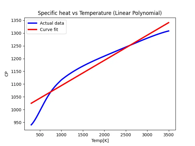
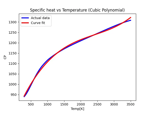
In linear polynomial, there is a noticeable difference as actual data deviates from the curve fit.

And in cubic polynomial, there is a subtle difference between the actual data and the curve fit.

• What needs to be done in order to make the curve fit perfect?

In order to make the curve fit perfectly, we should use the higher polynomial as we have seen from the previous results. The higher the polynomial, the more perfect the result will be.

• Show empirically as to how well your curve has been fit.

Following are codes of the few higher-order polynomials used to get the more perfect results.

# CURVE FITTING
# By Ajinkya Nikam

import math
import matplotlib.pyplot as plt 
import numpy as np
from scipy.optimize import curve_fit



# Curve fit function
def func(t, a, b, c, d, e):
	return a*pow(t,4) + b*pow(t,3) + c*pow(t,2) + d*t + e  


# Reading thermodynamic date file
def read_file():
	temp = []
	cp = []
	for line in open('Data', 'r'):
		values = line.split(',')
		temp.append(float(values[0]))
		cp.append(float(values[1]))
	return[temp , cp]

# Main Program

temp , cp = read_file()
popt, pcov = curve_fit(func, temp , cp)
fit_cp = func(np.array(temp), *popt)

plt.plot(temp , cp, color = "blue", linewidth = 3)
plt.plot(temp , fit_cp, color = "red", linewidth = 3)
plt.legend(['Actual data', 'Curve fit'])
plt.title('Specific heat vs Temperature(fourth order polynomial)')
plt.xlabel('Temp[K]')
plt.ylabel('CP')

plt.show()



#Curve fit function 
def func1(t, a, b, c, d, e, f):
	return a*pow(t, 5) + b*pow(t,4) + c*pow(t,3) + d*pow(t,2) + e*t + f  


# Reading thermodynamic data file
def read_file():
	temp = []
	cp = []
	for line in open('Data', 'r'):
		values = line.split(',')
		temp.append(float(values[0]))
		cp.append(float(values[1]))
	return[temp , cp]

# Main Program

temp , cp = read_file()
popt, pcov = curve_fit(func1, temp , cp)
fit_cp = func1(np.array(temp), *popt)

plt.plot(temp , cp, color = "blue", linewidth = 3)
plt.plot(temp , fit_cp, color = "red", linewidth = 3)
plt.legend(['Actual data', 'Curve fit'])
plt.title('Specific heat vs Temperature (fifth order Polynomial)')
plt.xlabel('Temp[K]')
plt.ylabel('CP')

plt.show()

Graphs:

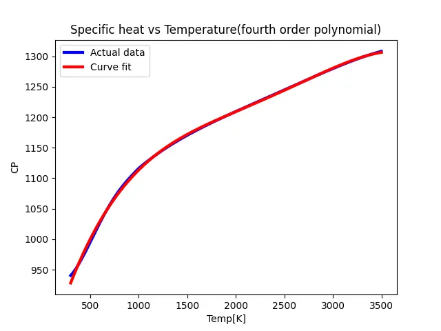
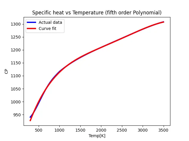
As you can see, as the order of polynomial goes higher, the more perfect the results are.