Week 2 Air standard Cycle
AIR STANDARD OTTO CYCLE:
AIM:
To create the program which will plot the actual P-V diagram of Air standard Otto cycle and to calculate the thermal efficiency at the different compression ratio.
Brief description of the governing equations of Air standard Otto cycle:
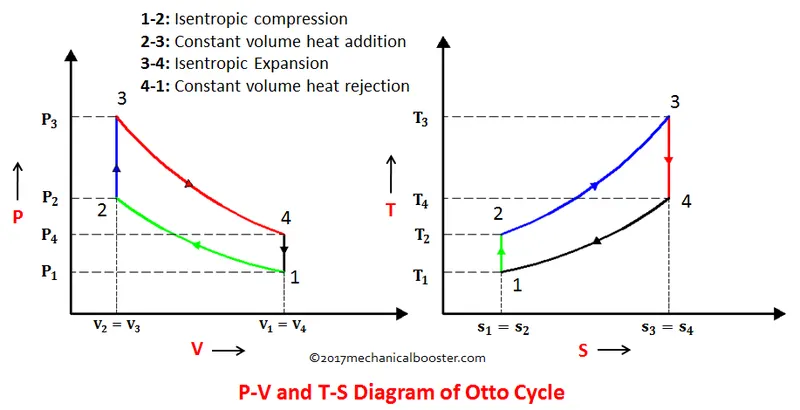
This is the cycle of most automobile engines and other four-stroke SI engines.
The air-standard-Otto cycle is the idealized cycle for the spark-ignition internal combustion engines. This cycle is shown above on p-v and T-s diagrams. The thermodynamic analysis of Otto cycle 1-2-3-4 consists of the following four processes:
Process 1-2: Isentropic compression of air.
Process 2-3: Heat addition at constant volume.
Process 3-4: Isentropic expansion of air.
Process 4-1: Heat rejection at constant volume.
Since processes 1-2 and 3-4 are adiabatic processes, the heat transfer during the cycle takes place only during processes 2-3 and 4-1 respectively. Therefore, the thermal efficiency can be written as,

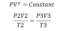
Following ideal gas equations are used to calculate the pressure and temperature:
Considered data to create the Otto cycle:
P1 = 101325 Pascal
T1 = 500°C
T3 =2300°C
Bore = 0.1m
Stroke = 0.1m
Connecting Rod = 0.15m
Compression Ratio = 12
Gamma = 1.4
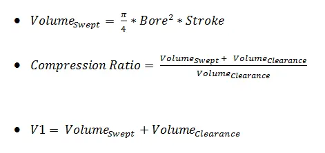
Given Equation:

Volume Calculations:
Objective:
The main objective of the project is to create the actual P-V diagram using the given data and to calculate the thermal efficiency of the Otto cycle and how it affects at different compression ratios.
The Brief Explanation of logic behind the code used:
- Firstly, we attributed the given data and gave the short names to the specific term to use for calculation. Afterward, by using the given data and ideal equation, we created the ideal Otto cycle. But as you know, the actual isentropic process doesn’t work linearly.
- Secondly, therefore, to create the actual cycle we defined our own function for the term like Bore, stroke, Compression Ratio, Start crank angle, End crank angle and we used it to perform the required specific task.
- At last, We used the array function to get the required amount of Compression ratio and plotted against the thermal efficiency.
Following are the codes used to get the ideal and actual Otto cycle:
Ideal Otto Cycle code:
""""
Basic Program of Ideal Otto cycle
"""
import math
import matplotlib.pyplot as plt

"""
We used the following thermodynamic analysis of Otto cycle to calculate the required parameters

Process 1-2: Isentropic compression of air.
Process 2-3: Heat addition at constant volume.
Process 3-4: Isentropic expansion of air.
Process 4-1: Heat rejection at constant volume.
"""

# State Point 1

P1 = 101325
T1 = 500
T3 =2300

#Geometric Parameters
Bore = 0.1
Stroke = 0.1
Conn_Rod = 0.15
CR = 12
gamma = 1.4

#Volume Calculations
V_s = math.pi*pow(Bore,2)/4     # Swept Volume
V_c = V_s/(CR-1)                # Clearance Volume
V1 = V_s + V_c


# State Point 2
V2 = V_c

# P1V1^gamma = P2V2^gamma
P2 = P1*pow(V1,gamma)/pow(V2,gamma)

# P1V1/T1 = P2V2/T2  |
RHS = P1*V1/T1
T2 = P2*V2/RHS

# State Point 3
V3 = V2

# P2V2/T2 = P3V3/T3
RHS = P2*V2/T2
P3 = RHS*T3/V3

#State point 4
V4 = V1

# P3V3^gamma = P4V4^gamma
P4 = P3*pow(V3, gamma)/pow(V4, gamma)

# P3V3/T3 = P4V4/T4
T4 = P4*V4/RHS


plt.plot([V1,V2,V3,V4,V1],[P1,P2,P3,P4,P1])

plt.title('P-V diagram of Ideal Air standard cycle')
plt.plot([V1,V2],[P1,P2], label = 'Isentropic Compression(1-2)', linewidth = 2)
plt.plot([V2, V3],[P2,P3], label = 'Constant Volume Heat Addition(2-3)', linewidth = 2)
plt.plot([V3, V4],[P3, P4], label = 'Isentropic Expansion(3-4)', linewidth = 2)
plt.plot([V4, V1], [P4, P1], label = 'Constant Volume Heat Rejection(4-1)', linewidth = 2)
plt.annotate("1", (V1, P1))
plt.annotate("2", (V2, P2))
plt.annotate("3", (V3, P3))
plt.annotate("4", (V4, P4))
plt.xlabel('Volume in m3')
plt.ylabel('Pressure in Pascal')
plt.show()
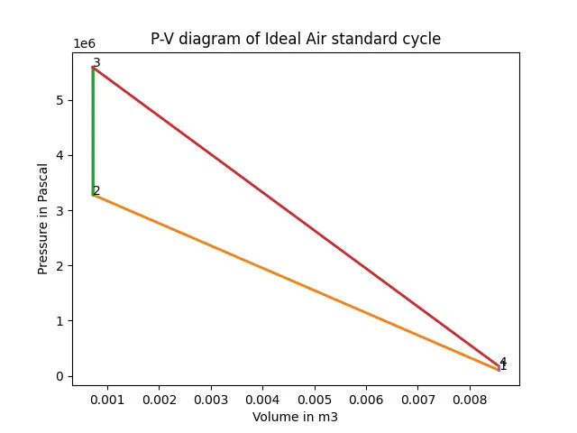
Graph of Ideal Otto Cycle:
Actual Otto Cycle code:
""""
Engine Kinematics
Program to create actual Otto cycle
by Ajinkya Nikam
"""
import math
import matplotlib.pyplot as plt

 # To perform the specific task and to make the code reusable, we defined our own function where we used 'def''

def Engine_Kinematics(Bore, Stroke, Conn_Rod, CR, Start_Crank_angle, End_Crank_angle):
	"""
	To create the function
	"""

	#Geometric Parameters

	a = Stroke/2
	R = Conn_Rod/a

	#Volume Calculations
	V_s = math.pi*pow(Bore,2)/4  # Swept volume
	V_c = V_s/(CR-1)             # Clearance volume

	S_C = math.radians(Start_Crank_angle)  # To get the angles in radian, we used the math.radian()
	E_C = math.radians(End_Crank_angle)

	Number_values = 100               # this value we can take as per the requirement,[ More the value more smooth your graph will be.]

	dtheta = (E_C - S_C)/(Number_values-1)

	V = []

	for i in range(0, Number_values):
		Theta = S_C + i*dtheta
		term1 = 0.5*(CR-1)
		term2 = R +1 -math.cos(Theta)
		term3 = pow(R, 2) - pow(math.sin(Theta), 2)
		term3 = pow(term3, 0.5)

		V.append(V_c*(1 + term1*(term2-term3)))
	return(V)

"""
We used the following thermodynamic analysis of Otto cycle to calculate the required parameters

Process 1-2: Isentropic compression of air.
Process 2-3: Heat addition at constant volume.
Process 3-4: Isentropic expansion of air.
Process 4-1: Heat rejection at constant volume.
"""

# State Point 1

P1 = 101325
T1 = 500
T3 =2300

#Geometric Parameters
Bore = 0.1
Stroke = 0.1
Conn_Rod = 0.15
CR = 12
gamma = 1.4

#Volume Calculations
V_s = math.pi*pow(Bore,2)/4
V_c = V_s/(CR-1)
V1 = V_s + V_c


# State Point 2
V2 = V_c

# P1V1^gamma = P2V2^gamma
P2 = P1*pow(V1,gamma)/pow(V2,gamma)

# Ideal Gas equation || P1V1/T1 = P2V2/T2  ||
RHS = P1*V1/T1
T2 = P2*V2/RHS
V_Compression = Engine_Kinematics(Bore, Stroke, Conn_Rod, CR, 0, 180)
Constant = P1*pow(V1, gamma)

P_Compression = []

for v in V_Compression:
	P_Compression.append(Constant/pow(v, gamma))

# State Point 3
V3 = V2

# P2V2/T2 = P3V3/T3
RHS = P2*V2/T2
P3 = RHS*T3/V3

V_Expanspion = Engine_Kinematics(Bore, Stroke, Conn_Rod, CR, 0, 180)
Constant = P3*pow(V3, gamma)

P_Expansion = []

for v in V_Expanspion:
	P_Expansion.append(Constant/pow(v, gamma))

#State point 4
V4 = V1

# P3V3^gamma = P4V4^gamma
P4 = P3*pow(V3, gamma)/pow(V4, gamma)

# P3V3/T3 = P4V4/T4
T4 = P4*V4/RHS

#Thermal efficiency of otto cycle

Thermal_Efficiency = 1 - ((T4 - T1)/(T3-T2))
print("Thermal_Efficiency = ",Thermal_Efficiency)


plt.plot(V_Compression, P_Compression)
plt.plot(V_Compression, P_Compression, label = 'Isentropic Compression(1-2)', linewidth = 2)
plt.plot([V2, V3],[P2,P3])
plt.plot([V2, V3],[P2,P3], label = 'Constant Volume Heat Addition(2-3)', linewidth = 2)
plt.plot(V_Expanspion, P_Expansion)
plt.plot(V_Expanspion, P_Expansion, label = 'Isentropic Expansion(3-4)', linewidth = 2)
plt.plot([V4, V1], [P4, P1])
plt.plot([V4, V1], [P4, P1], label = 'Constant Volume Heat Rejection(4-1)', linewidth = 2)
plt.title('P-V diagram of Actual Air Standard Cycle')
plt.annotate("1", (V1, P1))
plt.annotate("2", (V2, P2))
plt.annotate("3", (V3, P3))
plt.annotate("4", (V4, P4))
plt.xlabel('Volume in m3')
plt.ylabel('Pressure in Pascal')
plt.text(0.004,2*pow(10,6), 'Thermal Efficiency = 62.99%')
plt.legend()
plt.show()
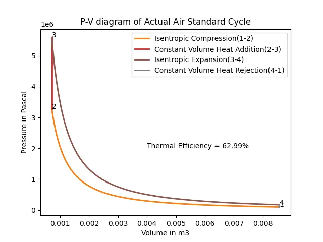
Graph of Actual Otto Cycle:
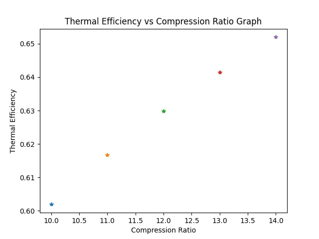
Following is the graph of thermal efficiency as compression ratio changes:
Code:
""""
Thermal efficiency vs Compression Ratio Graph
By Ajinkya Nikam
"""
import math
import matplotlib.pyplot as plt

# To create the otto cycle, we used the Function to perform the required task.

def Engine_Kinematics(Bore, Stroke, Conn_Rod, CR, Start_Crank_angle, End_Crank_angle):


	#Geometric Parameters

	a = Stroke/2
	R = Conn_Rod/a

	#Volume Calculations
	V_s = math.pi*pow(Bore,2)/4
	V_c = V_s/(CR-1)

	S_C = math.radians(Start_Crank_angle)
	E_C = math.radians(End_Crank_angle)

	Number_values = 100

	dtheta = (E_C - S_C)/(Number_values-1)

	V = []

	for i in range(0, Number_values):
		Theta = S_C + i*dtheta
		term1 = 0.5*(CR-1)
		term2 = R +1 -math.cos(Theta)
		term3 = pow(R, 2) - pow(math.sin(Theta), 2)
		term3 = pow(term3, 0.5)

		V.append(V_c*(1 + term1*(term2-term3)))

	return(V)


# State Point 1

P1 = 101325
T1 = 500
T3 =2300

#Geometric Parameters
Bore = 0.1
Stroke = 0.1
Conn_Rod = 0.15
gamma = 1.4

CRs = [10, 11, 12, 13, 14]

for i in CRs:
	CR = i
	#Volume Calculations
	V_s = math.pi*pow(Bore,2)/4
	V_c = V_s/(CR-1)
	V1 = V_s + V_c


	# State Point 2
	V2 = V_c

	# P1V1^gamma = P2V2^gamma
	P2 = P1*pow(V1,gamma)/pow(V2,gamma)

	# P1V1/T1 = P2V2/T2  |
	RHS = P1*V1/T1
	T2 = P2*V2/RHS
	V_Compression = Engine_Kinematics(Bore, Stroke, Conn_Rod, CR, 0, 180)
	Constant = P1*pow(V1, gamma)

	P_Compression = []

	for v in V_Compression:
		P_Compression.append(Constant/pow(v, gamma))

	# State Point 3
	V3 = V2

	# P2V2/T2 = P3V3/T3
	RHS = P2*V2/T2
	P3 = RHS*T3/V3

	V_Expanspion = Engine_Kinematics(Bore, Stroke, Conn_Rod, CR, 0, 180)
	Constant = P3*pow(V3, gamma)

	P_Expansion = []

	for v in V_Expanspion:
		P_Expansion.append(Constant/pow(v, gamma))

	#State point 4
	V4 = V1

	# P3V3^gamma = P4V4^gamma

	P4 = P3*pow(V3, gamma)/pow(V4, gamma)

	# P3V3/T3 = P4V4/T4
	T4 = P4*V4/RHS

	#Thermal efficiency of otto cycle

	Thermal_Efficiency = 1 - (T4 - T1)/(T3-T2)
	print("Thermal_Efficiency = ",Thermal_Efficiency)

	plt.plot(CR, Thermal_Efficiency,'*')
	plt.xlabel('Compression Ratio')
	plt.ylabel('Thermal Efficiency')
	plt.title('Thermal Efficiency vs Compression Ratio Graph')

plt.show()
"Thermal efficiency vs Compression ratio" Graph:
Conclusion:
- From the above observation and calculated output, we, clearly, can infer that the process of isentropic compression and expansion is not linear. And the area under the curve also differs between the Ideal and actual Otto cycle.
- As we can see in the thermal Efficiency vs Compression ratio graph, as the compression ratio goes up, thermal efficiency also goes up. The efficiency of the Otto cycle is mainly the function of compression ratio for the given gamma value i.e γ = Cp/Cv.