Week 5 - Curve fitting

1. What do 'popt' and 'pcov' mean?

The popt output argument is an array of the optimal values of coefficients for the polynomial we are using to fit the data.

The pcov output argument is a 2D array that contains the estimated covariance of the popt values with the original data.

2. What does np.array(temperature) do?

It converts a list in Python which is a linear data structure that can hold heterogeneous elements to an array which is a data structure that can hold homogeneous elements using the NumPy library.

3. What does the * in *popt mean?

The special syntax *args in function definitions in python is used to pass a variable number of arguments to a function. It is used to pass a non-key-worded, variable-length argument list.

4. Write code to fit a linear and cubic polynomial for the Cp data. Explain if your results are good or bad.

import math
import matplotlib.pyplot as plt 
import numpy as np 
from scipy.optimize import curve_fit

#curve fit functions - cubic and linear
def func1(t,a,b,c,d):
	return a*pow(t,3) + b*pow(t,2) + c*t + d 

def func2(t,e,f):
	return e*t + f

#Reading thermodynamic data file 
def read_file():
	temperature = []
	cp = []
	for line in open('data','r'):
		values = line.split(',')
		temperature.append(float(values[0]))
		cp.append(float(values[1]))
	return [temperature,cp]

#curve fitting 
temperature, cp = read_file()

popt1, pcov1 = curve_fit(func1, temperature, cp)
fit_cp1 = func1(np.array(temperature), *popt1)

popt2, pcov2 = curve_fit(func2, temperature, cp)
fit_cp2 = func2(np.array(temperature), *popt2)

#plotting 
plt.plot(temperature, cp,, linewidth = 3)
plt.plot(temperature, fit_cp1,, linewidth = 3)
plt.plot(temperature, fit_cp2,, linewidth = 3)

plt.legend(['Actual Data', 'Curve Fit Data(cubic)', 'Curve Fit Data(linear)'])
plt.xlabel('Temperature[K]')
plt.ylabel('Cp')
plt.show()

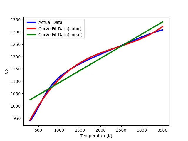
-> The output when a linear function is fit to the data is a straight line. It does not do justice to the actual characteristics of the data. Linearizing it oversimplifies the variation of data.

-> The cubic polynomial, when fit to the data produces a curve that better follows the actual data curve. Still, there are various points where the curve has large deviations from the actual data curve.

5. What needs to be done in order to make the curve fit perfectly?

-> Increasing the order of the polynomial could improve the fit to a certain extent.

-> The different sections of data can be assigned polynomials that best suit the nature of variation in that section. Hence, the data will be split and each section will be assigned a different polynomial.

6. Show empirically how well your curve has been fit.

-> Increasing the order of the polynomial could improve the fit to a certain extent.

import math
import matplotlib.pyplot as plt 
import numpy as np 
from scipy.optimize import curve_fit

#curve fit function - fourth degree polynomial
def func(t,a,b,c,d,e):
	return a*pow(t,4) + b*pow(t,3) + c*pow(t,2) + d*t + e 

#Reading thermodynamic data file 
def read_file():
	temperature = []
	cp = []
	for line in open('data','r'):
		values = line.split(',')
		temperature.append(float(values[0]))
		cp.append(float(values[1]))
	return [temperature,cp]

#curve fitting 
temperature, cp = read_file()
popt, pcov = curve_fit(func, temperature, cp)
fit_cp = func(np.array(temperature), *popt)

#plotting 
plt.plot(temperature, cp,, linewidth = 3)
plt.plot(temperature, fit_cp,, linewidth = 3)
plt.legend(['Actual Data', 'Curve Fit Data(4th deg poly)'])
plt.xlabel('Temperature[K]')
plt.ylabel('Cp')
plt.show()

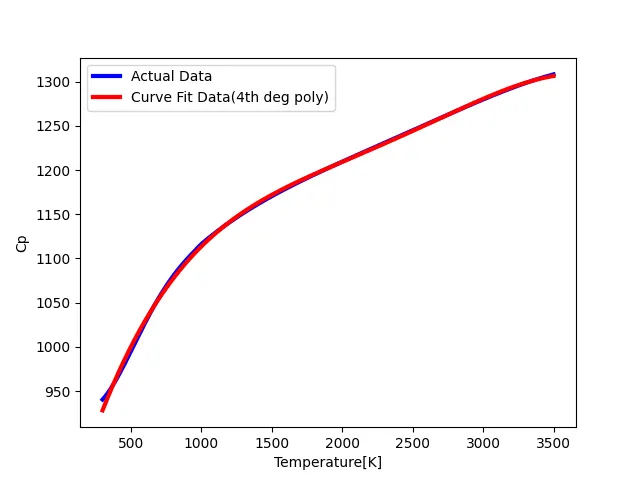
-> It is clearly visible how increasing the degree of the polynomial improves closeness of fit.

-> The different sections of data can be assigned polynomials that best suit the nature of variation in that section. Hence, the data will be split and each section will be assigned a different polynomial.

import math
import matplotlib.pyplot as plt 
import numpy as np 
from scipy.optimize import curve_fit

#curve fit functions - cubic and linear
def func1(t,a,b,c):
	return a*pow(t,2) + b*t + c

def func2(t,f,g):
	return f*t + g

#Reading thermodynamic data file 
def read_file():
	temperature = []
	cp = []
	for line in open('data','r'):
		values = line.split(',')
		temperature.append(float(values[0]))
		cp.append(float(values[1]))
	return [temperature,cp]

#curve fitting 
temperature, cp = read_file()

popt1, pcov1 = curve_fit(func2, temperature[0:450], cp[0:450])
fit_cp1 = func2(np.array(temperature[0:450]), *popt1)

popt2, pcov2 = curve_fit(func1, temperature[451:1200], cp[451:1200])
fit_cp2 = func1(np.array(temperature[451:1200]), *popt2)

popt3, pcov3 = curve_fit(func2, temperature[1201:3199], cp[1201:3199])
fit_cp3 = func2(np.array(temperature[1201:3199]), *popt3)

#plotting 
plt.plot(temperature, cp,, linewidth = 3)
plt.plot(temperature[0:450], fit_cp1,, linewidth = 3)
plt.plot(temperature[451:1200], fit_cp2,, linewidth = 3)
plt.plot(temperature[1201:3199], fit_cp3,, linewidth = 3)

plt.legend(['Actual Data', 'Curve Fit Data(cubic)', 'Curve Fit Data(linear)'])
plt.xlabel('Temperature[K]')
plt.ylabel('Cp')
plt.show()

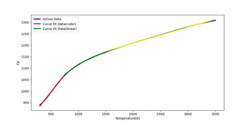
-> Dividing data into linear-quadratic-linear parts, improves closeness to fit as shown above.