Transient Motion Simulation of a Pendulum

Problem Statement:

Write a program in MATLAB to solve a second order 'Ordinary differential equation' that represents the equation of motion of a simple pendulum with damping and create an animation of this motion.

Theory :

The figure shows an idealized pendulum, with a "massless" string or rod of length 'L' and a bob of mass 'm'. When the bob is moved from its rest position and let go, it swings back and forth. The time it takes the pendulum to swing from its farthest right position to its farthest left position and back to its next farthest right position is the period of the pendulum. The primary forces acting on the bob are the gravitational force that makes it move in the first place and the force exerted by the string to keep it moving along a circular path. In addition, there may be a damping force from friction at the pivot or air resistance or both.

Mathematically the equation of motion of a simple pendulum wiht damping can be derived as -

Let theta(t) be the corresponding angle with respect to the vertical. The figure shows tangential and radial components of gravitational force on the pendulum bob. The radial component is exactly balanced by the force exerted by the string, so the only relevant force producing the motion is the tangential component of the gravitational force. For the moment, we ignore the damping force, if any.

The gravitational force is directed downward and has magnitude mg (mass x acceleration), where g is the gravitational acceleration constant 9.807 meters/sec2 near sea level. Thus, the force acting in the tangential direction is -mg sin(theta). (The negative sign is because this force is in the negative direction when theta is positive and vice versa.) Since this force is mass x acceleration, it follows that

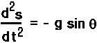
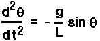
Now s and theta are related as arc length and central angle in a circle of radius L: s = L theta. Thus, the second derivative of s is L times the second derivative of theta. That brings us to our undamped model differential equation with a single dependent variable, the angular displacement theta:

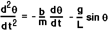
Next, we add damping to the model. We make the simplest possible assumption about the damping force, that it is proportional to velocity. Since arc length and central angle are themselves proportional (with proportionality constant L), it makes no difference whether we use linear or angular velocity. Having selected theta as our dependent variable, we will represent the damping as proportional to angular velocity, say, -b (d theta / dt). The negative sign is because the damping force has to be opposite the direction of motion. When we include this term in the model, our equation becomes

When we bring all the terms to the left-hand side, our model equation becomes -

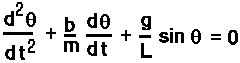
This equation is similar to the damped, unforced spring equation -

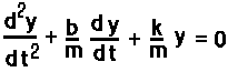
When these equations are solved, they are converted into two first order ODEs which are than converted to matrices. These matrices can be solved in MATLAB to obtain the velocity and displacement values with respect to time.

About the Program:

The most important part of the program is the ODE45 function that helps us solve the differential equation.

The function requires us to write code for a local function that can define the elements to be integrated.

function[dtheta_dt] = ode_func(t,theta,b,g,l,m) 

theta1 = theta(1);
theta2 = theta(2);
dtheta1_dt = theta2; %defining dtheta1_dt
dtheta2_dt = -(b/m)*theta2 - (g/l)*sin(theta1); %defining dtheta2_dt
[dtheta_dt] = [dtheta1_dt ; dtheta2_dt]; %converting to column matrix

end

This new function creates a column vector once the values of dtetha1_dt and dtetha2_dt are defined and assigns it to a solution vector dtetha_dt.

-----------------------------------------------------------------------------------------------------------------

clear all;
close all;
clc;
%solving 2nd order ODE to simulate transient Motion of a Pendulum

b = 0.4; %damping coefficient
l = 1; %length of string (m)
g = 9.8; %acceleration due to gravity (m/s^2)
m = 0.3; %mass of bob (Kg)

%intial parameters displacement = 0 and velocity = 5m/s
theta_0 = [0;5]; 

%time interval boundary conditions for ODE integration
tspan = linspace(0,10,500);

%calling the ODE45 function 

[t,results] = ode45(@(t,theta) ode_func(t, theta, b,g,l,m),tspan,theta_0);

%plotting
plot(t,results(:,1));
hold on;
plot(t,results(:,2));
xlabel('time');
ylabel('plot');
grid on;

->This program solves the second order ODE to create a plot showing the displacement and velocity variation with respect to time.

->The program takes damping coefficient, lenght of string, acceleration due to gravity, mass of bob, initial displacement and intial velocity as input parameters.

-> Timespan of 10 seconds is divided into 500 parts using linspace command to be used as boundary conditions for integration of the first order ODEs.

->plots created for time V/s displacement(results colum 1) and for time V/s velocity(results column 2)

Output -

-----------------------------------------------------------------------------------------------------------

clear all;
close all;
clc;

%solving 2nd order ODE to simulate transient Motion of a Pendulum

b = 0.4;  %damping coefficient
l = 1; %length of string (m)
g = 9.8; %acceleration due to gravity (m/s^2)
m = 0.3; %mass of bob (Kg)

%intial parameters displacement = 0 and velocity = 5m/s
theta_0 = [0;5];

%time interval boundary conditions for ODE integration
tspan = linspace(0,10,500);

%calling the ODE45 function
[t,results] = ode45(@(t,theta) ode_func(t, theta, b,g,l,m),tspan,theta_0);

%creating an array to store displacement values from 'results' array
disp_theta = results(:,1);

ct=1;%counter initiation
for i = 1:length(disp_theta) 
    THETA = disp_theta(i); 
    x0 = 0; %x & y coordinates of the fixed point of pendulum
    y0 = 0;
    
    x1 = l*cos((3*pi/2)+THETA); %x & y coordinates of bob
    y1 = l*sin((3*pi/2)+THETA);
    
    %plotting 
    plot([x0 x1],[y0 y1],'linewidth',3,'color','b');
    hold on
    plot(x1,y1,'o','MarkerFaceColor','r'); %to create the bob 
    hold on
    plot([-3 3],[0 0],'linewidth',3,'color','r'); %fixed point's base
    hold off
    axis([-3 3 -2 2])
    grid on;
    pause(0.03);
    K(ct)=getframe(gcf);%figure windows saved as frames in a struct array
    ct = ct+1;  % counter increment by 1  
end
movie(K) 
videofile = VideoWriter('Motion_of_Simple_Pendulum.avi','Uncompressed AVI');
open(videofile)
writeVideo(videofile,K)
close(videofile)

->after obtaining the results array, the displacement data is dumped into another array - 'disp_theta'.

->in the for loop coordinates of the fixed point of pendulum are fixed at (0,0) and the coordinates of the bob are evaluated using the displacement data from the results.

->These coordinates are then plotted to create the string and a marker is placed at the coordinates of the bob. 'movie' function is used to create a video out of the K(ct) structure array that obtains the figure window frames using the 'getframe' command. The 'VideoWriter' function allows us to create an output .avi format video.

Output-

Please use the following Youtube URL to watch the animation created using the above program -

https://youtu.be/8PbT9PV8i9k

Conclusions:

Motion of a simple pendulum can be simulated by solving such second order ODEs. The solutions show the effects of damping due to friction at joints and air stream. The function ODE45 allows us to solve ODE with time- and state-dependent mass matrix.