Week 5 - Curve fitting
Assignment 6
OBJECTIVE: The main objective of this challenge, is to write a python programme to fit Linear, Quadratic and Cubic polynomial for the Cp data. and to find the goodness of fit by using R-Square method.
PROBLEM STATEMENT:
In this assignment we have to find the goodness of fit for Linear, Quadratic and Cubic polynomial which have difficult methods to solve. Among this R-Square is prefered.
SOFTWARE USED:
Python3.6 (64bit), subline text3 as text editor.
THEORY:
Curve fitting is a type of optimization that finds an optimal set of parameters for a defined function that best fits a given set of observations.
Unlike supervised learning, curve fitting requires that you define the function that maps examples of inputs to outputs.
The mapping function, also called the basis function can have any form you like, including a straight line (linear regression), a curved line (polynomial regression), and much more. This provides the flexibility and control to define the form of the curve, where an optimization process is used to find the specific optimal parameters of the function.
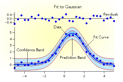
It is easiest to think about curve fitting in two dimensions, such as a graph.
Consider that we have collected examples of data from the problem domain with inputs and outputs.
The x-axis is the independent variable or the input to the function. The y-axis is the dependent variable or the output of the function. We don’t know the form of the function that maps examples of inputs to outputs, but we suspect that we can approximate the function with a standard function form.
Curve fitting involves first defining the functional form of the mapping function (also called the basis function or objective function), then searching for the parameters to the function that result in the minimum error.
Error is calculated by using the observations from the domain and passing the inputs to our candidate mapping function and calculating the output, then comparing the calculated output to the observed output.
Once fit, we can use the mapping function to interpolate or extrapolate new points in the domain. It is common to run a sequence of input values through the mapping function to calculate a sequence of outputs, then create a line plot of the result to show how output varies with input and how well the line fits the observed points.
The key to curve fitting is the form of the mapping function.
A straight line between inputs and outputs can be defined as follows:
- y = a * t + b
Where y is the calculated output, t is the input, and a and b are parameters of the mapping function found using an optimization algorithm.
This is called a linear equation because it is a weighted sum of the inputs.
In a linear regression model, these parameters are referred to as coefficients; in a neural network, they are referred to as weights.
This equation can be generalized to any number of inputs, meaning that the notion of curve fitting is not limited to two-dimensions (one input and one output), but could have many input variables.
For example, a line mapping function for two input variables may look as follows:
- y = a1 * t1 + a2 * t2 + b
The equation does not have to be a straight line.
We can add curves in the mapping function by adding exponents. For example, we can add a squared version of the input weighted by another parameter:
- y = a * t^2 + b * t + c
This is called polynomial regression, and the squared term means it is a second-degree polynomial.
So far, linear equations of this type can be fit by minimizing least squares and can be calculated analytically. This means we can find the optimal values of the parameters using a little linear algebra.
We can add curves in the mapping function by adding exponents. For example, we can add a cubic version of the input weighted by another parameter:
- y = a * t^3 + b * t^2 + c * t + d
This is called polynomial regression, and the cubic term means it is a third-degree polynomial.
4. Write code to fit a linear and cubic polynomial for the Cp data. Explain if your results are good or bad.
CASE-1 PROCEDURE: To write a python programme to fit Linear for the Cp data. And to find the goodness of fit by using R-Square method.
1. Open subline text editor.
2. Open a new file and save it as ----.py
3. Write the comment that what is the program is about, which the line is never executed. And write the comment first followed by #(pound) or double quotation codes in starting and as well as at the end of comments. then
import numpy as np
import matplotlib.pyplot as plt
from scipy.optimize import curve_fit
4. Define the Linear function
a * t + b + c
5. The thermodynamic file have to be read and in order to make the file readable, we have to save the readfile and the python program in the same folder.
def read_file():
6. Two unknowns such as temperature and the cp value have to be determined. In order to read the file we have to define both append and float command to the temperature and cp value.
temperature.append(float(values[0]))
cp.append(float(values[1]))
7. Include the popt and pcov in the program. popt contains the values for 'a' and 'b' and popt helps to refer the curve fit values. popt is a one dimensional array of the best estimates for the parameter values, each entry matches the order in the function definition. pcov is the covariance matrix showing the uncertainty and interdependence of each parameter in popt . We take the diagonal elements as pvar for the variance of each parameter in popt.
8. The model function needs to follow the curve_fit rules
The function must take and array of independent data as its first argument
The function can take any number of additional parameters that will be found using curve_fit
The function must return a single prediction of the dependent data for each value in the independent data.
9. FINDING R^2 VALUE SSR=SUM OF SQUARES OF REGRESSION, SSE = SUM OF SQUARES DUE TO ERROR
SSR_1 = np.array(cp) - np.mean(fit_cp)
SSR_2 = np.square(SSR_1)
SSR = sum(SSR_2)
SSE_1 = np.array(cp) - np.array(fit_cp)
SSE_2 = np.square(SSE_1)
SSE = sum(SSE_2)
SST = SSR+SSE
R_SQR = (SSR/SST)
10. PRINT and Plot the graph
print(R_SQR)
plt.plot(temperature, cp,, linewidth=3)
plt.plot(temperature, fit_cp,, linewidth=3)
plt.legend(['Actual data','Curve fit'])
plt.xlabel('temperature[K]')
plt.ylabel('cp')
plt.show()
PROGRAM SCREEN SHOT
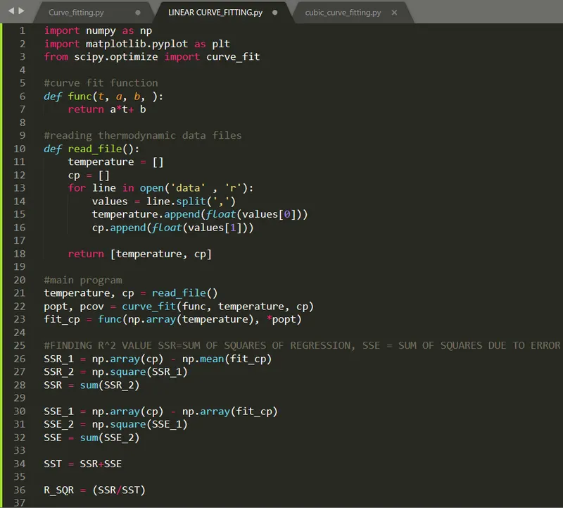
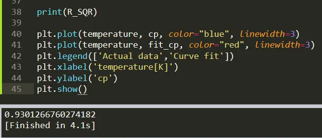
FIG PROGRAM
#LINEAR curve fit RENUKUMAR

import numpy as np
import matplotlib.pyplot as plt
from scipy.optimize import curve_fit

#curve fit function
def func(t, a, b, ):
	return a*t+ b

#reading thermodynamic data files
def read_file():
	temperature = []
	cp = []
	for line in open('data' , 'r'):
		values = line.split(',')
		temperature.append(float(values[0]))
		cp.append(float(values[1]))

	return [temperature, cp]

#main program
temperature, cp = read_file()
popt, pcov = curve_fit(func, temperature, cp)
fit_cp = func(np.array(temperature), *popt)

#FINDING R^2 VALUE SSR=SUM OF SQUARES OF REGRESSION, SSE = SUM OF SQUARES DUE TO ERROR
SSR_1 = np.array(cp) - np.mean(fit_cp)
SSR_2 = np.square(SSR_1)
SSR = sum(SSR_2)

SSE_1 = np.array(cp) - np.array(fit_cp)
SSE_2 = np.square(SSE_1)
SSE = sum(SSE_2)

SST = SSR+SSE

R_SQR = (SSR/SST)

print(R_SQR)

plt.plot(temperature, cp,, linewidth=3)
plt.plot(temperature, fit_cp,, linewidth=3)
plt.legend(['Actual data','Curve fit'])
plt.xlabel('temperature[K]')
plt.ylabel('cp')
plt.show()
CASE-2 PROCEDURE: To write a python programme to fit QUADRATIC Curve for the Cp data. And to find the goodness of fit by using R-Square method.
1. Open subline text editor.
2. Open a new file and save it as ----.py
3. Write the comment that what is the program is about, which the line is never executed. And write the comment first followed by #(pound) or double quotation codes in starting and as well as at the end of comments. then
import numpy as np
import matplotlib.pyplot as plt
from scipy.optimize import curve_fit
4. Define the Quadratic function
a * pow(t,2) + b * t + c
5. The thermodynamic file have to be read and in order to make the file readable, we have to save the readfile and the python program in the same folder.
def read_file():
6. Two unknowns such as temperature and the cp value have to be determined. In order to read the file we have to define both append and float command to the temperature and cp value.
temperature.append(float(values[0]))
cp.append(float(values[1]))
7. Include the popt and pcov in the program. popt contains the values for 'a' , 'b' and 'c'. popt helps to refer the curve fit values. popt is a one dimensional array of the best estimates for the parameter values, each entry matches the order in the function definition. pcov is the covariance matrix showing the uncertainty and interdependence of each parameter in popt . We take the diagonal elements as pvar for the variance of each parameter in popt.
8. The model function needs to follow the curve_fit rules
The function must take and array of independent data as its first argument
The function can take any number of additional parameters that will be found using curve_fit
The function must return a single prediction of the dependent data for each value in the independent data.
9. FINDING R^2 VALUE SSR=SUM OF SQUARES OF REGRESSION, SSE = SUM OF SQUARES DUE TO ERROR
SSR_1 = np.array(cp) - np.mean(fit_cp)
SSR_2 = np.square(SSR_1)
SSR = sum(SSR_2)
SSE_1 = np.array(cp) - np.array(fit_cp)
SSE_2 = np.square(SSE_1)
SSE = sum(SSE_2)
SST = SSR+SSE
R_SQR = (SSR/SST)
10. PRINT and Plot the graph
print(R_SQR)
plt.plot(temperature, cp,, linewidth=3)
plt.plot(temperature, fit_cp,, linewidth=3)
plt.legend(['Actual data','Curve fit'])
plt.xlabel('temperature[K]')
plt.ylabel('cp')
plt.show()
PROGRAM SCREEN SHOT
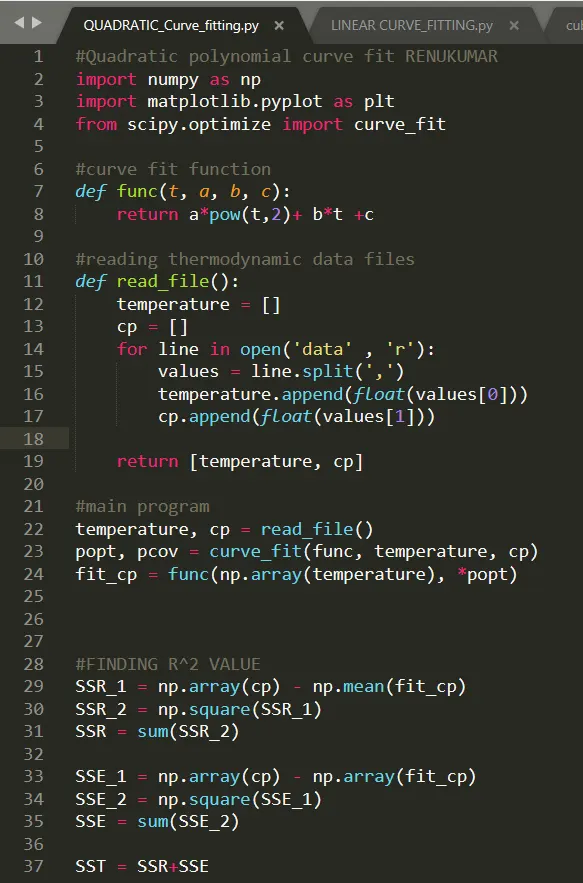
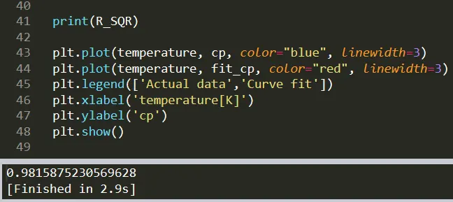
FIG PROGRAM
#Quadratic polynomial curve fit RENUKUMAR
import numpy as np
import matplotlib.pyplot as plt
from scipy.optimize import curve_fit

#curve fit function
def func(t, a, b, c):
	return a*pow(t,2)+ b*t +c

#reading thermodynamic data files
def read_file():
	temperature = []
	cp = []
	for line in open('data' , 'r'):
		values = line.split(',')
		temperature.append(float(values[0]))
		cp.append(float(values[1]))

	return [temperature, cp]

#main program
temperature, cp = read_file()
popt, pcov = curve_fit(func, temperature, cp)
fit_cp = func(np.array(temperature), *popt)


#FINDING R^2 VALUE
SSR_1 = np.array(cp) - np.mean(fit_cp)
SSR_2 = np.square(SSR_1)
SSR = sum(SSR_2)

SSE_1 = np.array(cp) - np.array(fit_cp)
SSE_2 = np.square(SSE_1)
SSE = sum(SSE_2)

SST = SSR+SSE

R_SQR = (SSR/SST)

print(R_SQR)

plt.plot(temperature, cp,, linewidth=3)
plt.plot(temperature, fit_cp,, linewidth=3)
plt.legend(['Actual data','Curve fit'])
plt.xlabel('temperature[K]')
plt.ylabel('cp')
plt.show()
CASE-3 PROCEDURE: To write a python programme to fit CUBIC Curve for the Cp data. And to find the goodness of fit by using R-Square method.
1. Open subline text editor.
2. Open a new file and save it as ----.py
3. Write the comment that what is the program is about, which the line is never executed. And write the comment first followed by #(pound) or double quotation codes in starting and as well as at the end of comments. then
import numpy as np
import matplotlib.pyplot as plt
from scipy.optimize import curve_fit
4. Define the Cubic function
a * pow(t,3) + b * pow(t,2) + c * t + d
5. The thermodynamic file have to be read and in order to make the file readable, we have to save the readfile and the python program in the same folder.
def read_file():
6. Two unknowns such as temperature and the cp value have to be determined. In order to read the file we have to define both append and float command to the temperature and cp value.
temperature.append(float(values[0]))
cp.append(float(values[1]))
7. Include the popt and pcov in the program. popt contains the values for 'a' , 'b' , 'c' and 'd'. popt helps to refer the curve fit values. popt is a one dimensional array of the best estimates for the parameter values, each entry matches the order in the function definition. pcov is the covariance matrix showing the uncertainty and interdependence of each parameter in popt . We take the diagonal elements as pvar for the variance of each parameter in popt.
8. The model function needs to follow the curve_fit rules
The function must take and array of independent data as its first argument
The function can take any number of additional parameters that will be found using curve_fit
The function must return a single prediction of the dependent data for each value in the independent data.
9. FINDING R^2 VALUE SSR=SUM OF SQUARES OF REGRESSION, SSE = SUM OF SQUARES DUE TO ERROR
SSR_1 = np.array(cp) - np.mean(fit_cp)
SSR_2 = np.square(SSR_1)
SSR = sum(SSR_2)
SSE_1 = np.array(cp) - np.array(fit_cp)
SSE_2 = np.square(SSE_1)
SSE = sum(SSE_2)
SST = SSR+SSE
R_SQR = (SSR/SST)
10. PRINT and Plot the graph
print(R_SQR)
plt.plot(temperature, cp,, linewidth=3)
plt.plot(temperature, fit_cp,, linewidth=3)
plt.legend(['Actual data','Curve fit'])
plt.xlabel('temperature[K]')
plt.ylabel('cp')
plt.show()
PROGRAM SCREEN SHOT
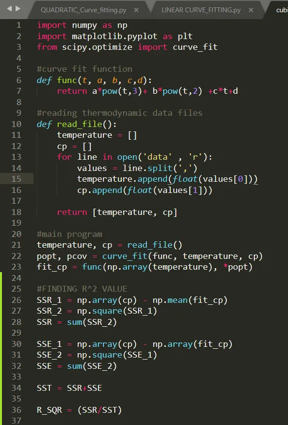
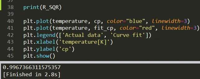
FIG PROGRAM
# CUBIC CURVE FITTING RENU KUMAR

import numpy as np
import matplotlib.pyplot as plt
from scipy.optimize import curve_fit

#curve fit function
def func(t, a, b, c,d):
	return a*pow(t,3)+ b*pow(t,2) +c*t+d

#reading thermodynamic data files
def read_file():
	temperature = []
	cp = []
	for line in open('data' , 'r'):
		values = line.split(',')
		temperature.append(float(values[0]))
		cp.append(float(values[1]))

	return [temperature, cp]

#main program
temperature, cp = read_file()
popt, pcov = curve_fit(func, temperature, cp)
fit_cp = func(np.array(temperature), *popt)

#FINDING R^2 VALUE
SSR_1 = np.array(cp) - np.mean(fit_cp)
SSR_2 = np.square(SSR_1)
SSR = sum(SSR_2)

SSE_1 = np.array(cp) - np.array(fit_cp)
SSE_2 = np.square(SSE_1)
SSE = sum(SSE_2)

SST = SSR+SSE

R_SQR = (SSR/SST)

print(R_SQR)

plt.plot(temperature, cp,, linewidth=3)
plt.plot(temperature, fit_cp,, linewidth=3)
plt.legend(['Actual data', 'Curve fit'])
plt.xlabel('temperature[K]')
plt.ylabel('cp')
plt.show()
RESULT:
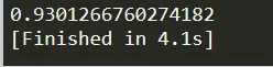
FOR THE LINEAR FUNCTION THE VALUE OF R-SQUARE IS
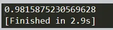
FOR THE QUADRATIC FUNCTION THE VALUE OF R-SQUARE IS
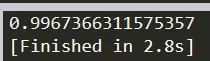
FOR THE CUBIC FUNCTION THE VALUE OF R-SQUARE IS
GRAPH: OUT PUT
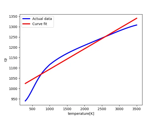
LINEAR CURVE FIT
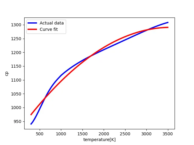
QUADRATIC CURVE FIT
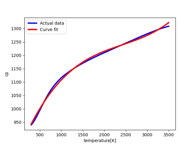
CUBIC CURVE FIT
QUESTION AND ANSWERS
1. What does popt and pcov mean? (Watch the video to get some context)
ANS popt contains the values for 'a' , 'b' , 'c' and 'd'. popt helps to refer the curve fit values. popt is a one dimensional array of the best estimates for the parameter values, each entry matches the order in the function. pcov is the covariance matrix showing the uncertainty and interdependence of each parameter in popt . We take the diagonal elements as pvar for the variance of each parameter in popt.
2. What does np.array(temperature) do?
ANS The function of np.array(temperature) is to pass the entire temperatures through the function which is defined in the program as well as the popt.The value of temperatures are saved in the data file which is copied in the same program folder.
3. What does the * in *popt mean?
ANS POPT is used to find the optimum coefficients for the data set. where as * refers to the cp and temperature in the function.
5. What needs to be done in order to make the curve fit perfect?
ANS In order to make the curve fit perfect as in the order of polynomial, the error will increase and a phenomina called as the over fit is taking place. By splitting the order we can make the curve fit perfect.
6. Show empirically as to how well your curve has been fit.
ANS Empirically means obervation or experience, by oberving the below graphs we can say that the cubic curve fit is well when compared to quadratic curve fit, similarly the quadratic curve fit is well when compared to the linear curve fit.
LINEAR CURVE FIT QUADRATIC CURVE FIT CUBIC CURVE FIT
RESULT AND DISCUSSION:
FOR THE LINEAR FUNCTION THE VALUE OF R-SQUARE IS 0.9301266760274182
FOR THE QUADRATIC FUNCTION THE VALUE OF R-SQUARE IS 0.9815875230569628
FOR THE CUBIC FUNCTION THE VALUE OF R-SQUARE IS 0.9967366311575357
R-Square ranges from a value of 0-1
0 for the worst possible fit for the data set
1 for the best possible fit for the data set
From the above values we can see that the cubic function will be very close to the value of 1, which is treated as best possible fit. Among this function the cubic function is very close to the best value when compared to quadratic function, similarly quadratic function is very close to the best value when compared to linear function.
Difficulty faced
We had faced the difficulty while understanding the concept of R-Square method, support engineer makes it easy to understand and results are plotted.
LINK: https://drive.google.com/drive/folders/1Ni9u6DtihyDz8v0U33g2lLVZUdE6S0zV?usp=sharing