Week 5 - Curve fitting

Curve fitting:-

curve fitting is a process of constructing a curve that has the closest similarity for the series of data being considered. Curve fitting examines the relationship between one and more predictors and a response variable with the defining the best model.

The curve fit is classified into 3 types:

1. Linear regression
2. Polynomial regression
3. Logistic regression

Regression is a technique used to find the trends of the data, by this technique we will predict the data by using the equations.

The best fit can be chosen by 4different methods:

1. Sum of Squares due to Error (SSE)
2. R-square
3. Adjusted R-square
4. Root Mean Squared Error (RMSE)

The value of R-square is calculated by using the following formula:

`R^2 = (SSR)/(SST)`

SSR = sum of squares of regression

SST = SSR + SSE

Curve fit can be made perfect by interpolating the database, by interpolating the errors can be minimized. The linear, quadratic, cubic, and split-wise curve fit codes are given below:

Linear polynomial: Y = `Ax + B`

Quadratic polynomial: Y = `Ax^2 + Bx + C`

Cubic polynomial: Y = `Ax^3 + Bx^2 + Cx + D`

Initially, we are writing the code for linear, quadratic, and cubic polynomial and check the results with original plots.

• popt:- This command gives an array with the optimal values for the parameters so that the sum of the squared residuals of data is minimized.
• pcov:- This command is a 2D array with the estimated covariance of the parameters in popt. It can be used to calculate the standard deviation errors of popt.
• np.array(temperature):- This function stores the values of the temperature in the form of the array and it passes through a function numpy.
• *in* popt:- It stores the values of the constant parameters in the array popt. The * indicates the function will accept the arguments supplied in the function that r not identified in the list.
• To make a curve fit perfect the error estimates should be considered. The perfect fit is a fit where it should match the original curve and shouldn't have any scaling and centering errors in that particular degree of the polynomial. The R^2 value must be equal to 1 and SSE=0.
• We can fit the curve by increasing the degree of the polynomial or splitting the curve into different parts by using splitwise method.

Code:-

import math  # for doing mathamatical calculations
import matplotlib.pyplot as plt  # for ploting
import numpy as np # numpy is used to +, -, *, /, power, and linspace for the arrays
from scipy.optimize import curve_fit

'''
	curve fit for linear polynomial
'''

# linear curve fit   
def fun(t,a,b,):
	return a*t + b

# reading thermodynamic data file
def read_file():
	temperature = []
	cp = []
	for line in open('data','r'):
		values = line.split(',')
		temperature.append(float(values[0]))
		cp.append(float(values[1]))

	return [temperature, cp]	 


# Main program
temperature, cp = read_file()
popt, pcov = curve_fit(fun, temperature, cp)
fit_cp = fun(np.array(temperature),*popt)

plt.plot(temperature, cp,color='blue',linewidth=2)
plt.plot(temperature, fit_cp,color='red',linewidth=2)
plt.title('Linear method for Specific heat Vs Temperature')
plt.legend(['Actual data','Curve fit'])
plt.xlabel('Temperature[k]')
plt.ylabel('Specific heat(cp)')
plt.grid('on')
plt.show()


'''
	curve fit for Quadratic polynomial
'''

# Quadratic curve fit
def func(t,a,b,c):
	return a*pow(t,2) + b*t + c

# reading thermodynamic data file
def read_file():
	temperature = []
	cp = []
	for line in open('data','r'):
		values = line.split(',')
		temperature.append(float(values[0]))
		cp.append(float(values[1]))

	return [temperature, cp]	 


# Main program
temperature, cp = read_file()
popt, pcov = curve_fit(func, temperature, cp)
fit_cp = func(np.array(temperature),*popt)

plt.plot(temperature, cp,color='blue',linewidth=2)
plt.plot(temperature, fit_cp,color='red',linewidth=2)
plt.title('Quadratic method for Specific heat Vs Temperature')
plt.legend(['Actual data','Curve fit'])
plt.xlabel('Temperature[k]')
plt.ylabel('Specific heat(cp)')
plt.grid('on')
plt.show()


'''
	curve fit for cubic polynomial
'''

# Cubic curve fit
def fun(t,a,b,c,d):
	return a*pow(t,3) + b*pow(t,2) + c*t + d

# reading thermodynamic data file
def read_file():
	temperature = []
	cp = []
	for line in open('data','r'):
		values = line.split(',')
		temperature.append(float(values[0]))
		cp.append(float(values[1]))

	return [temperature, cp]	 


# Main program
temperature, cp = read_file()
popt, pcov = curve_fit(fun, temperature, cp)
fit_cp = fun(np.array(temperature),*popt)

plt.plot(temperature, cp,color='blue',linewidth=2)
plt.plot(temperature, fit_cp,color='red',linewidth=2)
plt.title('Cubic method for Specific heat Vs Temperature')
plt.legend(['Actual data','Curve fit'])
plt.xlabel('Temperature[k]')
plt.ylabel('Specific heat(cp)')
plt.grid('on')
plt.show()

Result:-

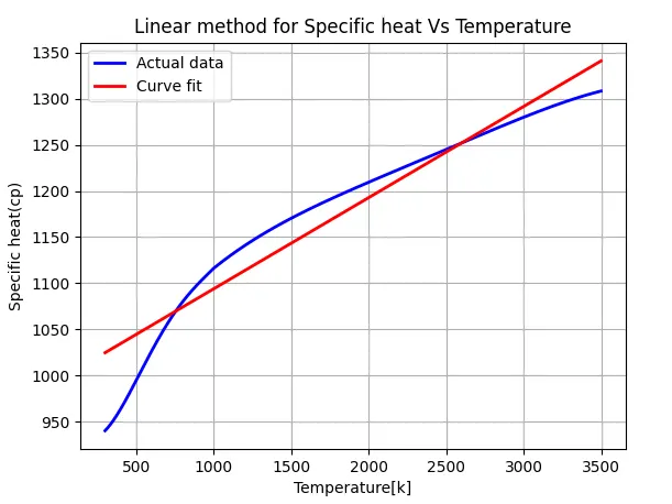
For Linear curve fit:

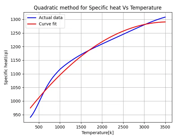
For Quadratic curve fit:

For Cubic curve fit:

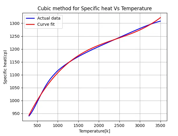
From the above plots, the curve fit is better with the increase in the degree of the polynomial. If we consider the fourth and fifth polynomial then we will get the perfect curve fit.

Or in other words, we can get the perfect curve fit by using the splitwise polynomial method.

For splitwise curve fit the SSE = 0(worst possible fit) and max R-square = 1(perfect possible fit), and for the linear curve fit the SSE is high and low `R^2` and for Cubic curve fit the SSE is low and high `R^2`.