Week 5 - Curve fitting

1. What does popt and pcov mean?

popt: it is command from scipy.optimize's curve_fit function which calculates the optimal coefficients for the equation at hand.

pcov: it is command from scipy.optimize's curve_fit function which calculates the covariance between two points. Covaraince is a quantity which determines the extent to which two variables vary simulaneously. Covariance is analogous to variance, but variance determines the variation of a single variable.

2. What does np.array(temperature) do?

The actual data is initially read and is stored in array format. For performing curve fit along with the actual curve, the temeprature and specific heats for the curve fit should be in array format as well, else there will be a mismatch in the plots. Hence, the temperature for curve approximation is fed in an array format.

3. What does the * in *popt mean?

popt calculates the optimal coefficients for the equation. The "*" in *popt is used to refer the coefficients from popt calculation and pass it to each value of temperature present in the array.

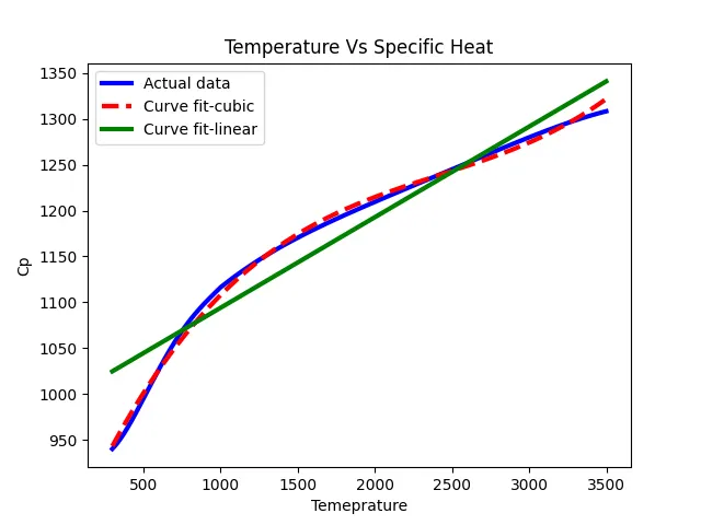
4. Write code to fit a linear and cubic polynomial for the Cp data. Explain if your results are good or bad.

Code:

# Curve fitting with linear and cubic polynomial
import math
import matplotlib.pyplot as plt
from scipy.optimize import curve_fit
import numpy as np

# Reading data from the temperature and Cp file
def read_file():
	temperature = []
	Cp = []
	for line in open('data', 'r'):
		values = line.split(',')
		temperature.append(float(values[0]))
		Cp.append(float(values[1]))

	return [temperature, Cp]

# Reading Temperature and Cp Values
temperature, Cp = read_file()

# Linear variation
def linear(temperature, a, b):
	return a*temperature + b

# Curve fitting program
popt, pcov = curve_fit(linear, temperature, Cp)
fit_Cp_linear = linear(np.array(temperature), *popt)

# Cubic variation
def cubic(t, a, b, c, d):
	return a*pow(t, 3) + b*pow(t, 2) + c*t + d

# Curve fitting program
popt, pcov = curve_fit(cubic, temperature, Cp)
fit_Cp_cubic = cubic(np.array(temperature), *popt)

plt.plot(temperature, Cp, '-', color = "blue", linewidth = 3)
plt.plot(temperature, fit_Cp_cubic, '--', color = "red", linewidth = 3)
plt.plot(temperature, fit_Cp_linear, '-', color = "green", linewidth = 3)
plt.legend(['Actual data', 'Curve fit-cubic', 'Curve fit-linear'])
plt.xlabel('Temeprature')
plt.ylabel('Cp')
plt.title('Temperature Vs Specific Heat')
plt.show()

Results and Discussion:

With linear curve fit, the deviation between the actual and the fit curve is significantly high. Linear fit represents an inappropriate approximation. Whereas, with cubic polynomial, the fit is comparatively closer. But still deviates at the point of inflection and at the end of the curve.

5. What needs to be done in order to make the curve fit perfect?

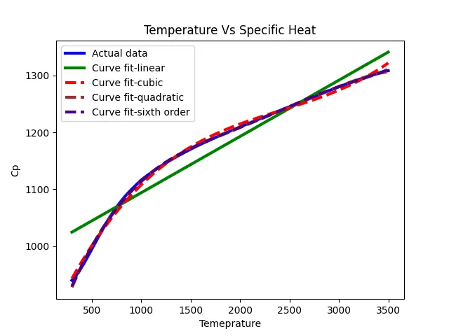
There are two ways which can improve the fit of approximated curve with the actual curve:

a. By increasing the degree of polynomial of the approximated curve. Increasing the degree of polynomial increases the approximation percentage.

Code:

# Perform curve fitting with different degrees of polynomial
import math
import matplotlib.pyplot as plt
import numpy as np
from scipy.optimize import curve_fit

def read_file():
	temperature = []
	Cp = []
	for line in open('data','r'):
		values = line.split(',')
		temperature.append(float(values[0]))
		Cp.append(float(values[1]))

	return [temperature, Cp]

# Linear curve fit function
def linear(t, a, b):
	return a*t + b

# Reading original values of data
temperature, Cp = read_file()

# Linear fit calculation
popt, pcov = curve_fit(linear, temperature, Cp)
fit_Cp_linear = linear(np.array(temperature), *popt)


def cubic(t, a, b, c, d):
	return a*pow(t ,3) + b*pow(t, 2) + c*t + d

# cubic fit calculation
popt, pcov = curve_fit(cubic, temperature, Cp)
fit_Cp_cubic = cubic(np.array(temperature), *popt)

def quadratic(t, a, b, c, d, e):
	return a*pow(t, 4) + b*pow(t, 3) + c*pow(t, 2) + d*t + e

# quadratic fit calculation
popt, pcov = curve_fit(quadratic, temperature, Cp)
fit_Cp_quadratic = quadratic(np.array(temperature), *popt)

# Sixth order
def sixth_order(t, a, b, c, d, e, f, g):
	return a*pow(t, 6) + b*pow(t, 5) + c*pow(t, 4) + d*pow(t, 3) + e*pow(t, 2) + f*t + g

# sixth order fit calculation
popt, pcov = curve_fit(sixth_order, temperature, Cp)
fit_Cp_sixth = sixth_order(np.array(temperature), *popt)


plt.plot(temperature, Cp, '-', color = "blue", linewidth = 3)
plt.plot(temperature, fit_Cp_linear, '-', color = "green", linewidth = 3)
plt.plot(temperature, fit_Cp_cubic, '--', color = "red", linewidth = 3)
plt.plot(temperature, fit_Cp_quadratic, '--', color = "brown", linewidth = 3)
plt.plot(temperature, fit_Cp_sixth, '--', color = "indigo", linewidth = 3)
plt.legend(['Actual data', 'Curve fit-linear', 'Curve fit-cubic','Curve fit-quadratic','Curve fit-sixth order'])
plt.xlabel('Temeprature')
plt.ylabel('Cp')
plt.title('Temperature Vs Specific Heat')
plt.show()

Plot:

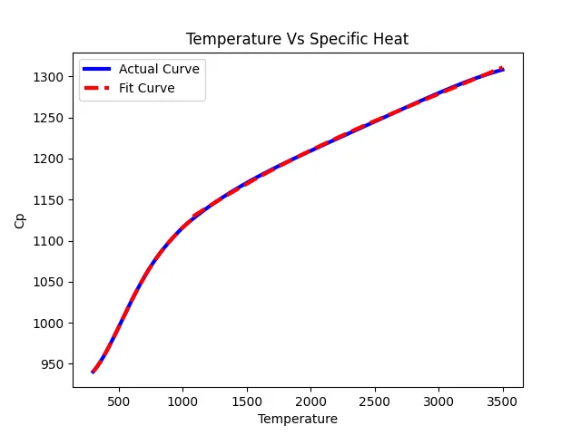
b. Split the dataset into subgroups and perform curve fit.

Splitting the dataset into subsets and then fitting gives a much closer fit to the actual curve.

Code:

# Curve fitting by splitting the dataset
import math
import matplotlib.pyplot as plt
import numpy as np
from scipy.optimize import curve_fit

def read_file():
	tempretaure = []
	Cp = []
	for line in open('data', 'r'):
		values = line.split(',')
		tempretaure.append(float(values[0]))
		Cp.append(float(values[1]))

	return [tempretaure, Cp]

# Defining a cubic function for curve fitting
def cubic(t, a, b, c, d):
	return a*pow(t ,3) + b*pow(t, 2) + c*t + d

# Main Program
# Read Temperature and Cp values
tempretaure, Cp = read_file()

"""
		Splitting the dataset in three subgroups
"""
# Group 1
tempretaure300_699 = tempretaure[0:400]
Cp300_699 = Cp[0:400]
tempretaure1 = np.linspace(300, 699, 398)
popt, pcov = curve_fit(cubic, tempretaure300_699, Cp300_699) # calculating the arguments for group 1
fit_Cp300_699 = cubic(np.array(tempretaure1), *popt) # Fitting Cp with the calculated arguments for group 1

# Group 2
temperature700_1079 = tempretaure[400:780]
Cp700_1079 = Cp[400:780]
temperature2 = np.linspace(700, 1079, 379)
popt, pcov = curve_fit(cubic, temperature700_1079, Cp700_1079) # calculating the arguments for group 2
fit_Cp700_1079 = cubic(np.array(temperature2), *popt) # Fitting Cp with the calculated arguments for group 1

# Group 3
temperature1080_3499 = tempretaure[780:3200]
Cp1080_3200 = Cp[780:3200]
temperature3 = np.linspace(1080, 3499, 2420)
popt, pcov = curve_fit(cubic, temperature1080_3499, Cp1080_3200) # calculating the arguments for group 3
fit_Cp1080_3499 = cubic(np.array(temperature3), *popt) # Fitting Cp with the calculated arguments for group 1

# Plotting
plt.plot(tempretaure, Cp, '-', color = "blue", linewidth = 3)
plt.plot(tempretaure1, fit_Cp300_699, '--', color = "red", linewidth = 3)
plt.plot(temperature2, fit_Cp700_1079, '--', color = "red", linewidth = 3)
plt.plot(temperature3, fit_Cp1080_3499, '--', color = "red", linewidth = 3)
plt.xlabel("Temperature")
plt.ylabel("Cp")
plt.legend(["Actual Curve", "Fit Curve"])
plt.title("Temperature Vs Specific Heat")
plt.show()

Plot: