Python for Mechanical Engineers

Week 5 - Curve fitting

Curve fitting can be defined as the process of constructing a curve or mathematical function that has the best fit to a series of data points, subject to constraints.

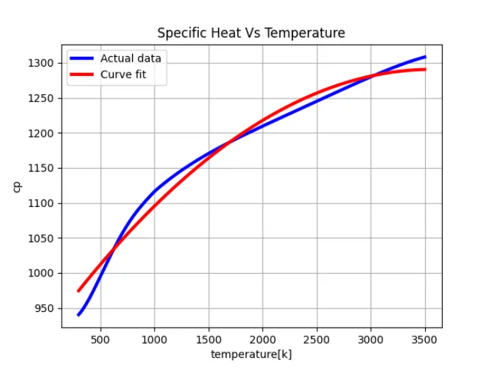
In this project, the curve for Specific heat as a function of Temperature will be plotted and the plot will be compared with the actual plot.

The specific heats at different temperatures will be provided as inputs.

Initially, we will be writing a program for linear and cubic polynomial and check the results with the actual plot. Based on the results obtained, we are going to figure out the best possible ways to have a perfect fit.

popt: It gives an array with the optimal values for the parameters so that the sum of the squared residuals of data is minimized

pcov: It is a 2d array with the estimated covariance of the parameters in popt. It can be used to calculate the the standard deviation errors of popt.

np.array(temperature): This function stores the values of temperature in the form of array and passes it to the function numpy.

* in *popt: It stores the values of the constant parameters(a,b,c) in the array popt.

Program:

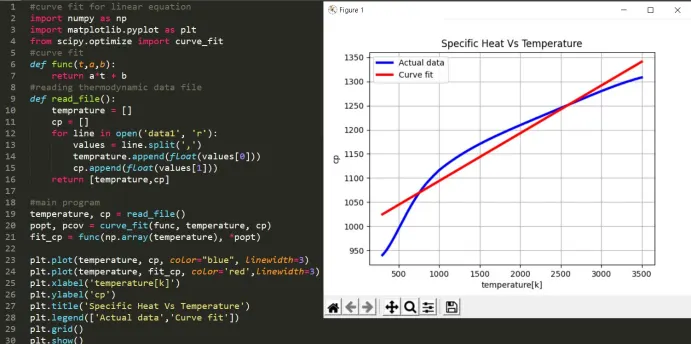
#curve fit for linear equation
import numpy as np 
import matplotlib.pyplot as plt 
from scipy.optimize import curve_fit
#curve fit
def func(t,a,b):
	return a*t + b
#reading thermodynamic data file
def read_file():
	temprature = []
	cp = []
	for line in open('data1', 'r'):
		values = line.split(',')
		temprature.append(float(values[0]))
		cp.append(float(values[1]))
	return [temprature,cp]

#main program
temperature, cp = read_file()
popt, pcov = curve_fit(func, temperature, cp)
fit_cp = func(np.array(temperature), *popt)

plt.plot(temperature, cp,, linewidth=3)
plt.plot(temperature, fit_cp, color='red',linewidth=3)
plt.xlabel('temperature[k]')
plt.ylabel('cp')
plt.title('Specific Heat Vs Temperature')
plt.legend(['Actual data','Curve fit'])
plt.grid()
plt.show()

#curve fit for quadratic equation
import numpy as np 
import matplotlib.pyplot as plt 
from scipy.optimize import curve_fit
#curve fit
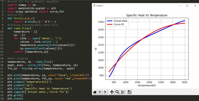
def func(t,a,b,c):
	return a*pow(t,2) + b*t + c
#reading thermodynamic data file
def read_file():
	temprature = []
	cp = []
	for line in open('data1', 'r'):
		values = line.split(',')
		temprature.append(float(values[0]))
		cp.append(float(values[1]))
	return [temprature,cp]

#main program
temperature, cp = read_file()
popt, pcov = curve_fit(func, temperature, cp)
fit_cp = func(np.array(temperature), *popt)

plt.plot(temperature, cp,, linewidth=3)
plt.plot(temperature, fit_cp, color='red',linewidth=3)
plt.xlabel('temperature[k]')
plt.ylabel('cp')
plt.title('Specific Heat Vs Temperature')
plt.legend(['Actual data','Curve fit'])
plt.grid()
plt.show()
		

#curve fit for cubic equation
import numpy as np 
import matplotlib.pyplot as plt 
from scipy.optimize import curve_fit
#curve fit
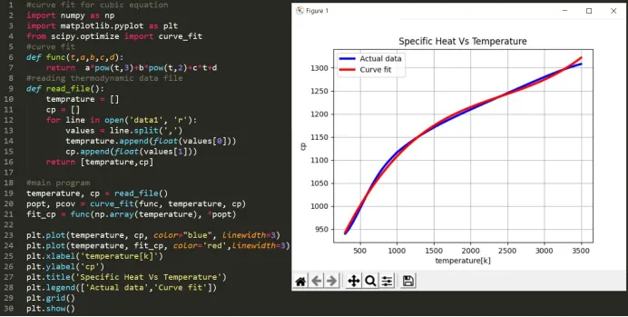
def func(t,a,b,c,d):
	return  a*pow(t,3)+b*pow(t,2)+c*t+d 
#reading thermodynamic data file
def read_file():
	temprature = []
	cp = []
	for line in open('data1', 'r'):
		values = line.split(',')
		temprature.append(float(values[0]))
		cp.append(float(values[1]))
	return [temprature,cp]

#main program
temperature, cp = read_file()
popt, pcov = curve_fit(func, temperature, cp)
fit_cp = func(np.array(temperature), *popt)

plt.plot(temperature, cp,, linewidth=3)
plt.plot(temperature, fit_cp, color='red',linewidth=3)
plt.xlabel('temperature[k]')
plt.ylabel('cp')
plt.title('Specific Heat Vs Temperature')
plt.legend(['Actual data','Curve fit'])
plt.grid()
plt.show()

Results:

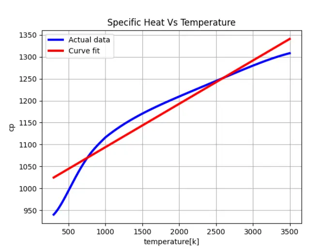
Linear curve fit:

Quadratic Curve fit:

Cubic Curve fit:

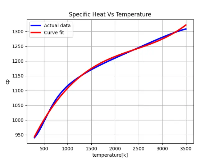
It is clear from the above figures that the curve fits better when the degree of the polynomial increases. It can be observed that the deviation of the curve fit with the actual data is more for linear equation and gradually the deviation decreases with the increase in the order of the polynomial. If we consider fourth, fifth order polynomials etc then the curve fit will overlap with the actual data.