Week 5 - Curve fitting

1. What does popt & pcov mean?

popt : array

Optimal value for the parameters so that the sum of the squared residuals of given data is minimzed

pcov : 2d array

The estimated covarience of popt.the diagonals provide the variance of the parameter estimate

pcov variables contains the covariance matrix, which indicates the uncertainties & correlations between parameters. This is mostly useful when the data has uncertainities.

2.What does np.array(temperature) do?

The numpy array function converts list of values into array of the same size & with the same type of values.

3. What does the * in *popt mean?

* reference to the values stored in the array of popt (The * notation will expand a list of values into the arguments of the function. This is useful if the function has more than one (or) two parameters.

4. Write code to fit a linear & cubic polynomial for the cp data. Explain if your results are good or bad?

Code for Linear Polynomial:

import numpy as np
import matplotlib.pyplot as plt
from scipy.optimize import curve_fit

# Curve fit function
def func(t, a, b):
	return a*t+b

# Reading thermodynamic data file
def read_file():
	temperature = []
	cp = []
	for line in open('data','r'):
		values = line.split(',')
		temperature.append(float(values[0]))
		cp.append(float(values[1]))

	return [temperature, cp]

# Main program
temperature,cp = read_file()
popt, pcov = curve_fit(func,temperature,cp)
fit_cp = func(np.array(temperature), *popt)

plt.plot(temperature,cp,color="blue",linewidth=3)
plt.plot(temperature, fit_cp,color="red",linewidth=3)
plt.legend(['Actual data','curve fit-linear'])
plt.xlabel('Temperature [k]')
plt.ylabel('cp')
plt.show()

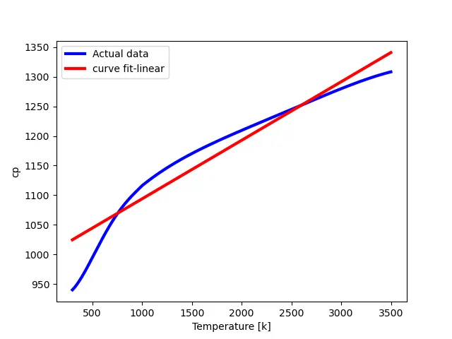
Output image of linear fit of the data

Code for the Cubic Polynomial:

import numpy as np
import matplotlib.pyplot as plt
from scipy.optimize import curve_fit

# Curve fit function
def func(t, a, b, c, d):
	return a*pow(t,3)+b*pow(t,2)+c*t+d

# Reading thermodynamic data file
def read_file():
	temperature = []
	cp = []
	for line in open('data','r'):
		values = line.split(',')
		temperature.append(float(values[0]))
		cp.append(float(values[1]))

	return [temperature, cp]

# Main program
temperature,cp = read_file()
popt, pcov = curve_fit(func,temperature,cp)
fit_cp = func(np.array(temperature), *popt)

plt.plot(temperature,cp,color="blue",linewidth=3)
plt.plot(temperature, fit_cp,color="orange",linewidth=3)
plt.legend(['Actual data','curve fit - cubic'])
plt.xlabel('Temperature [k]')
plt.ylabel('cp')
plt.show()

Output image of Cubic fit of the data:

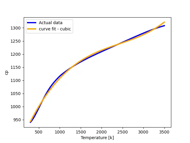
The linear function is not correctly approximate for the data it was given to fit. A straight line will not be suitable.

A cubic polynomial function manages to follow the trend of the data closer than the straight line.

Cubic fit is better than the linear fit.

5. What needs to be done in order to make the curve fit perfect?

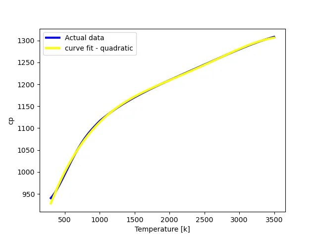
By increasing the degree of order the curve is getting the curve fit the approximate curve fit

It is obivious that higher the order of the polynomial, better will be the fit.

4th order polynomial curve fit 5th order polynomial curve fit

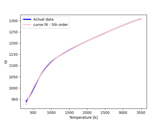
To fit a curve perfectly split-wise curve fitting method is required to used for perfect fit

6. Show empirically as to how well your curve has been fit.

Code: Split-wise polynomial curve fitting function:

import numpy as np
import matplotlib.pyplot as plt
from scipy.optimize import curve_fit

# Curve fit function
def func1(t, a, b, c):
	return a*pow(t,2)+b*t+c

def func2(t, a, b, c, d):
	return a*pow(t,3)+b*pow(t,2)+c*t+d

def func3(t, a, b, c, d, e):
	return a*pow(t,4)+b*pow(t,3)+c*pow(t,2)+d*t+e

def func4(t, a, b, c, d, e, f):
	return a*pow(t,5)+b*pow(t,4)+c*pow(t,3)+d*pow(t,2)+e*t+f

# Reading thermodynamic data file
def read_file():
	temperature = []
	cp = []
	for line in open('data','r'):
		values = line.split(',')
		temperature.append(float(values[0]))
		cp.append(float(values[1]))

	return [temperature, cp]

# Main program
temperature,cp = read_file()

#splitting the data into ranges
# Temperature from 300-600
t300_600=temperature[:300]
cp300_600=cp[:300]

t1 = np.linspace(300,600,300)
popt, pcov = curve_fit(func1,t300_600,cp300_600)
fit300_600 = func1(np.array(t1), *popt)

# Temperature from 600-1000
t600_1000=temperature[300:700]
cp600_1000=cp[300:700]

t2 = np.linspace(600,1000,400)
popt, pcov = curve_fit(func2,t600_1000,cp600_1000)
fit600_1000 = func2(np.array(t2), *popt)

# Temperature from 1000-2000
t1000_2000=temperature[700:1700]
cp1000_2000=cp[700:1700]

t3 = np.linspace(1000,2000,1000)
popt, pcov = curve_fit(func3,t1000_2000,cp1000_2000)
fit1000_2000 = func3(np.array(t3), *popt)

# Temperature from 600-1000
t2000=temperature[1700:]
cp2000=cp[1700:]

t4 = np.linspace(2000,3500,1500)
popt, pcov = curve_fit(func4,t2000,cp2000)
fit2000 = func4(np.array(t4), *popt)

plt.plot(temperature,cp,color="blue",linewidth=4)
plt.plot(t1,fit300_600,color="orange",linewidth=3)
plt.plot(t2,fit600_1000,color="red",linewidth=3)
plt.plot(t3,fit1000_2000,color="pink",linewidth=3)
plt.plot(t4,fit2000,color="yellow",linewidth=3)
plt.legend(['Actual data','curve fit - quadratic','curve fit - cubic','curve fit - 4th degree','curve fit - 5th degree'])
plt.xlabel('Temperature [k]')
plt.ylabel('cp')
plt.show()

Output image of split-wise curve fit:

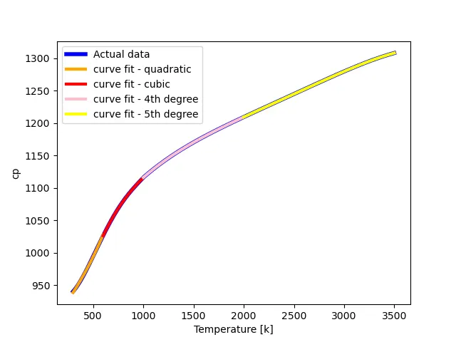
By considering the above graph we can say that slpit wise curve fit is gives the curve fit perfect.