Week 3 - Solving second order ODEs

Aim :- To write a program for second order differential equation to simulate the transient behavior of the simple pendulum.

Objective :-

1. To solve the 2nd ODE of motion of the simple pendulum with damping
2. To simulate the motion between 0-20sec to animate the motion of pendulum

Theory :-

A simple pendulum consists of a mass m hanging from a string of length L and fixed at a pivot point P. When displaced to an initial angle and released, the pendulum will swing back and forth with periodic motion.

The way of pendulum moves depends on the Newtons Second law. When this law is written down, we get a second order differential equation that describes the position of the "ball" w.r.t time.

Procedure :-

PYTHON code:-

import numpy as np
from scipy.integrate import odeint
import matplotlib.pyplot as plt
import math

# Function that returns dz/dt
def model(theta, t, b, g, l, m):

	theta1 = theta[0]
	theta2 = theta[1]
	dtheta1_dt = theta2
	dtheta2_dt = -(b/m)*theta2 - (g/l)*math.sin(theta1)
	dtheta_dt = [dtheta1_dt, dtheta2_dt]
	return dtheta_dt

b=0.05
g=9.81
l=1
m=1

#initial condition
theta_0 = [0,3]

# time points
t = np.linspace(0,20,150)

# solve ODE
theta = odeint(model,theta_0,t,args = (b,g,l,m))

#plot results
plt.plot(t,theta[:,0],'b-',label=r'$\frac{d\theta_1}{dt}=\theta_2$')
plt.plot(t,theta[:,1],'r--',label=r'$\frac{d\theta_2}{dt}=-\frac{b}{m}\theta_2-\frac{g}{l}sin\theta_1$')
plt.xlabel('plot')
plt.ylabel('time')
plt.legend(loc='best')
plt.show()

ct = 1
x1 = 0
y1 = 0

n = 150
for i in range (0,n):

	x2=x1+1*math.sin(theta[i,0])
	y2=y1-1*math.cos(theta[i,0])
	filename = 'pendulum%05d.png' % ct
	plt.figure()
	plt.plot([-1.5,1.5],[0,0],linewidth = 5)
	plt.plot([x1,x2],[y1,y2],linewidth = 4)
	plt.plot(x2,y2,marker='o',markersize = '10')
	plt.xlim(-1.5,1.5)
	plt.ylim(-1.5,1.5)
	plt.savefig(filename)
	ct=ct+1

Output:-

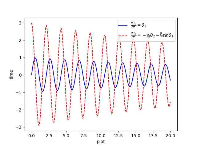
Plot that describes the variation of displacement and velocity w.r.t time.

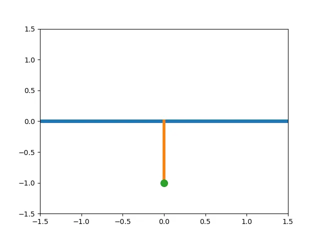
Animation of the motion of pendulum