Week 5 - Curve fitting

Aim

To perform curve fitting of the given data file using a program created by using python and determining the best fit for the given data file set.

Curve fitting

1. Perfect Curve fit

The perfect fit can be achieved only when the geometric distances from the given points to the fitting curve is zero. This implies that the curve fits perfectly with the data points provided. So in order to get a perfect fit, we can increase the degree of the polynomial as a result of which this method increases the accuracy and reduces the errors encountered.

The idea behind raising the overall order of the equation is to achieve the value of R^2 as 1. The criteria for the perfect fit is that the value of the R^2 value is 1.

2. Best fit

The best fit during the curve fit is achieved when the geometric distances from the given points to the fitting curve is minimized, in the least square sense. Finding the best fit reduces the minimization of the objective function.

The best fit can be achieved by the following methods:

• To increase the degree of the polynomial.
• To use the split wise method shown in the project
• To use the curve split toolbox in Matlab.

The goodness of fit can be measured by the following methods:

1. The sum of squares due to error (SSE).
2. R- square.
3. Adjusted R- Square.
4. Root mean squared error (RMSE)

Usually, if the R square is greater than 0.95 the fit is considered to be Best.

And if the value of R square is 1 then the curve fit is considered to be perfect

3.Improvement in the cubic fit method

The cubic fit can be improved by using the split wise method in which the curve is split into multiple numbers of polynomials for different sets of temperature values.

It can also be improved by reducing the error between the original dataset and curve fit value.

The main factor in splitting the data is the number of divisions/splits. By ensuring more splits of the data a higher accuracy of the output curve can be achieved.

Objectives

1. To do the curve fitting of the given data set of temperature and coefficient of pressure using a python code
2. To determine the goodness of the curve fit.

Questions in the challenge

1. What does popt and pcov mean?

Ans:-

• popt- This is an array containing the coefficients of the polynomial specified at the beginning of the program.
• pcov- This is a square matrix that contains the true variance and covariance of the parameters.

2. What does np.array(temperature) do?

Ans:-

This command creates an array of temperatures from the values stored in a data file using the numpy module.

3. What does the * in *popt mean?

Ans-

This command in the program refers to the coefficients of the polynomial into consideration during the running of the program.

4. Write code to fit a linear and cubic polynomial for the Cp data. Explain if your results are good or bad.

Ans-

The code of the program is given below in the project after the question answers.

5. What needs to be done in order to make the curve fit perfect?

Ans-

The best fit during the curve fit is achieved when the geometric distances from the given points to the fitting curve is minimized, in the least square sense. Finding the best fit reduces the minimization of the objective function.

The best fit can be achieved by the following methods:

• To increase the degree of the polynomial.
• To use the split wise method shown in the project
• To use the curve split toolbox in Matlab.

The goodness of fit can be measured by the following methods:

1. The sum of squares due to error (SSE).
2. R- square.
3. Adjusted R- Square.
4. Root mean squared error (RMSE)

Usually, if the R square is greater than 0.95 the fit is considered to be Best.

And if the value of R square is 1 then the curve fit is considered to be perfect

6. Show empirically as to how well your curve has been fit.

Ans-

This is achieved by using the various plots achieved using the execution of the program and then using the values of R generated in the command terminal. If it is greater than 0.95 then it's considered best and if it is equal to 1 then the curve fit is considered to be perfect.

Python code

"""
Python program for the curve fitting of the given data file

"""
import numpy as np 
import matplotlib.pyplot as plt 
from scipy.optimize import curve_fit

# the functions for the curve fit
def f_1(t,a,b):
	return a*t + b

def f_2(t,a,b,c):
	return a*pow(t,2) + b*t +c

def f_3(t,a,b,c,d):
	return a*pow(t,3)+b*pow(t,2)+c*t+d

def f_4(t,a,b,c,d,e):
	return a*pow(t,4)+b*pow(t,3)+c*pow(t,2)+d*t +e

# initialization of the data file given

def read_file():
	temperature=[]
	cp=[]
	for line in open ('data','r'):
		values=line.split(',')
		temperature.append(float(values[0]))
		cp.append(float(values[1]))

	return [temperature,cp]

# Curve fit part
temperature,cp=read_file()

#linear fit
popt,pcov=curve_fit(f_1,temperature,cp)
fit_cp_1=f_1(np.array(temperature), *popt)

# linear fit plot

plt.figure(1)
plt.plot(temperature,cp,'k-',linewidth=2)
plt.plot(temperature,fit_cp_1,color='magenta',linewidth=3)
plt.legend(['Actual data','Curve Fit'])
plt.title('Linear curve fit')
plt.xlabel('Temperature [K]')
plt.ylabel('Cp')
plt.show()

# Quad curve fit
popt,pcov=curve_fit(f_2,temperature,cp)
fit_cp_2=f_2(np.array(temperature), *popt)

#Quad fit plot
plt.figure(2)
plt.plot(temperature,cp,'k-',linewidth=2)
plt.plot(temperature,fit_cp_2,color='green',linewidth=3)
plt.legend(['Actual data','Curve Fit'])
plt.title('Quad curve fit')
plt.xlabel('Temperature [K]')
plt.ylabel('Cp')
plt.show()

# Cubic curve fit
popt,pcov=curve_fit(f_3,temperature,cp)
fit_cp_3=f_3(np.array(temperature), *popt)

# Cubic fit plot
plt.figure(3)
plt.plot(temperature,cp,'k-',linewidth=2)
plt.plot(temperature,fit_cp_3,color='red',linewidth=3)
plt.legend(['Actual data','Curve Fit'])
plt.title('Cubic curve fit')
plt.xlabel('Temperature [K]')
plt.ylabel('Cp')
plt.show()

# Bi quad curve fit
popt,pcov=curve_fit(f_4,temperature,cp)
fit_cp_4=f_4(np.array(temperature), *popt)

# Bi quad fit plot
plt.figure(4)
plt.plot(temperature,cp,'k-',linewidth=2)
plt.plot(temperature,fit_cp_4,color='blue',linewidth=3)
plt.legend(['Actual data','Curve Fit'])
plt.title('Cubic curve fit')
plt.xlabel('Temperature [K]')
plt.ylabel('Cp')
plt.show()

# Checking the qulaity of fit
s=np.sum(cp)
n=np.size(cp)

m=s/n #mean

# for linear curve fit
SSR_lin=0
SSE_lin=0

for i in range (n):
	error=abs((np.sum((cp[i]-fit_cp_1[i]))))
	SSE_lin=SSE_lin+pow(error,2)
	SSR_lin=SSR_lin+(np.sum(pow(fit_cp_1[i]-m,2)))

SST_lin=SSE_lin+SSR_lin
Rsq_lin=SSR_lin/SST_lin
RMSE_lin=pow((SSE_lin/n),0.5)

print('SST_lin:',SST_lin)
print('Rsq_lin:',Rsq_lin)
print('RMSE_lin:',RMSE_lin)

# for quad curve fit
SSR_quad=0
SSE_quad=0

for i in range (n):
	error=abs((np.sum((cp[i]-fit_cp_2[i]))))
	SSE_quad=SSE_quad+pow(error,2)
	SSR_quad=SSR_quad+(np.sum(pow(fit_cp_2[i]-m,2)))

SST_quad=SSE_quad+SSR_quad
Rsq_quad=SSR_quad/SST_quad
RMSE_quad=pow((SSE_quad/n),0.5)

print('SST_quad:',SST_quad)
print('Rsq_quad:',Rsq_quad)
print('RMSE_quad:',RMSE_quad)

# for cubic fit
SSR_cubic=0
SSE_cubic=0

for i in range (n):
	error=abs((np.sum((cp[i]-fit_cp_3[i]))))
	SSE_cubic=SSE_cubic+pow(error,2)
	SSR_cubic=SSR_cubic+(np.sum(pow(fit_cp_3[i]-m,2)))

SST_cubic=SSE_cubic+SSR_cubic
Rsq_cubic=SSR_cubic/SST_cubic
RMSE_cubic=pow((SSE_cubic/n),0.5)

print('SST_cubic:',SST_cubic)
print('Rsq_cubic:',Rsq_cubic)
print('RMSE_cubic:',RMSE_cubic)

# for bi quad curve fit

SSR_bq=0
SSE_bq=0

for i in range (n):
	error=abs((np.sum((cp[i]-fit_cp_4[i]))))
	SSE_bq=SSE_bq+pow(error,2)
	SSR_bq=SSR_bq+(np.sum(pow(fit_cp_4[i]-m,2)))

SST_bq=SSE_bq+SSR_bq
Rsq_bq=SSR_bq/SST_bq
RMSE_bq=pow((SSE_bq/n),0.5)

print('SST_bq:',SST_bq)
print('Rsq_bq:',Rsq_bq)
print('RMSE_bq:',RMSE_bq)

Working of code

1. First, the various models are imported as per the various calculations involved in the program
2. After the importing of the modules, the various functions are defined on the basis of which the various polynomial fit of the curve is carried out. These are linear, quadratic, cubic, and biquadratic functions which are defined as per the general mathematical definition.
3. Then the command is given for reading the data file by the program for the extraction of the required data of temperature and coefficient of pressure.
4. After this under each type of function by using pot and pcov commands functions and curve fit already defined under scipy module of the python library is carried out.
5. After this, for each function, separate plot commands are given after the curve fit command for each type of function.
6. After this, the goodness of the curve fit is determined by using the equations for manual calculations of the required parameters.
7. These equations calculate the values for SST, RMSE, and R^2 for the evaluation of the goodness of the curve fit

Plots

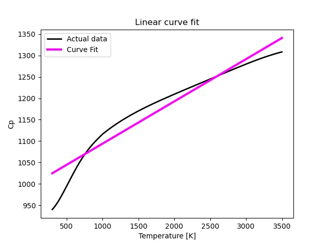
• Linear fit
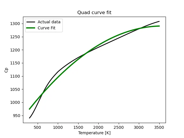
• Quadratic fit
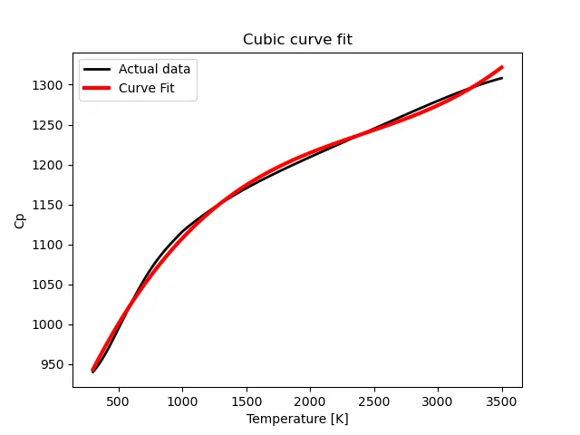
• Cubic Fit
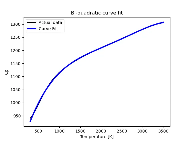
• Bi-quadratic fit

Errors

• Apart from the normal syntax error for plotting purposes, there were no major errors encountered during the coding of this project.

Results

• The linear fit for the given data is not sufficient and hence higher level of the curve fit should be obtained.
• The quadratic fit as per the plot also doesn't match the data set correctly hence higher-order curve fit is required to be obtained
• The cubic fit shows a good accuracy but not the best accuracy as per the plot hence higher-order curve fit is opted for.
• The biquadratic curve fit is the best fit as per the plot obtained hence the curve fit for higher order is not continued further.
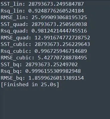
• After the final study of the empirical calculation, the biquadratic curve fit appears as best as per the value of R^2.
• The values of SST, R^2, and RMSE for the empirical comparison is given as follows

Conclusion:

The curve fitting of the given data file using a program created by using python and determining the best fit for the given data file set has been successfully completed.