Week 5 - Curve fitting

AIM : To write code to fit a linear and cubic polynomial for the Cp data given and to find answers for the following questions :-

1. What does popt and pcov mean?

2. What does np.array(temperature) do?

3. What does the * in *popt mean?

4. What needs to be done in order to make the curve fit perfect?

THEORY : The given data file contains the data of variuos temperatures corresponding to different values of cp.

The general form of a linear polynomial is :

ax + b

The general form of a cubic polynomial is :

ax^3 + bx^2 + cx + d

Where a, b, c, d are various coefficients of the polynomial.

PROCEDURE :

import numpy as np 
import matplotlib.pyplot as plt 
from scipy.optimize import curve_fit

def func1(x,a,b,c,d):
	return a*pow(x,3) + b*pow(x,2) + c*x + d 
 
def func2(x,a,b):
	return a*x + b

def read_file():
	temperature = []
	cp = []
	for line in open('data','r'):
		values = line.split(',')
		temperature.append(float(values[0]))
		cp.append(float(values[1]))
	return [temperature,cp]

temperature,cp = read_file()
popt_1,pcov_1 = curve_fit(func1,temperature,cp)
popt_2,pcov_2 = curve_fit(func2,temperature,cp)
fit_cp_1 = func1(np.array(temperature),*popt_1)
fit_cp_2 = func2(np.array(temperature),*popt_2)

plt.plot(temperature,cp,color = 'green',linewidth = 2)
plt.plot(temperature,fit_cp_1,color = 'red',linewidth = 2)
plt.plot(temperature,fit_cp_2,color = 'blue',linewidth = 2)
plt.legend(['Actual fit', 'Curve fit for cubic polynomial','Curve fit for linear polynomial'])
plt.xlabel('Temperature [K]')
plt.ylabel('cp')

plt.show()

Firstly the required modules were imported for us to use the methods from them later in the program.

Then two different functions were defined, one which returns a cubic polynomial, and the other returns a linear polynomial.

Then a function called read_file was created which reads the data file available and sorts the temperature and cp values into seperate elements of a list called values.

Then each of the value of temperature and cp in the list 'values' is assigned to empty lists called temperature and cp respectively.

Then, by calling the function read_file, values are assigned to the variables temperature and cp outside of the function definition.

Then using the curve_fit method from the scipy module, best parameters for the coefficients a,b,c,d in the case of cubic polynomial, and a,b in the case of linear polynomial are assigned with the argument 'popt'.

The pcov variable contains the covariance matrix, which indicates the uncertainties and correlations between parameters.

Then a variable called 'fit_cp', one for each of the polynomial, is assigned the respective polynomials with the help of the the command " func(np.array(temperature),*popt)".

Here, np.array converts the values stored in the variable temperature into an array or a list, which are then assigned the values of the parameters stored in popt with the help of "*".

Later using the matplotlib module, curves are plotted for the actual curve, curve for the linear polynomial and curve for the cubic polynomial.

RESULT :

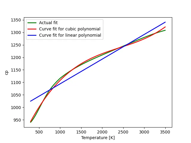
And it can be noticed that the cubic polynomail curve is more accurate than the curve of linear polynomial with regards to the actual curve. So it can be said that as the degree of the polynomial increases, the accuracy of the curve fitting also increases.

CONCLUSION :

The code to fit a linear and cubic polynomial for the Cp data was succesfully written and the questions asked in the aim were answered while explaining the procedure.