Curve fitting

1. What do popt and pcov mean?

popt: It gives an array with the optimal values for the parameters so that the sum of the squared residuals of data is minimized.

pcov: It is a 2d array with the estimated covariance of the parameters in popt. It can be used to calculate the standard deviation errors of popt.

2. What does np.array(temperature) do?

Np.array(temperature): This function stores the values of the temperature in the form of an array and passes it to the function numpy. Numpy is a Python library that is the core library for scientific computing in Python.np.array(temperature) creates a ray with the value present in the temperature variable.

3. What does the * in *popt mean?

*in*popt: it stores the values of the constant parameters(a,b,c) in the array popt.

Theory

Curve fitting is the process of constructing a curve or mathematical function, that has the best fit to a series of data points, possibly subject to constraints. Curve fitting can involve either interpolation, where an exact fit to the data is required, or smoothing, in which a "smooth" function is constructed that approximately fits the data.

A related topic is regression analysis, which focuses more on questions of statistical inference such as how much uncertainty is present in a curve that is fit to data observed with random errors.

Fitted curves can be used as an aid for data visualization, to infer values of a function where no data are available, and to summarize the relationships among two or more variables.

The goodness of Fit is decided based on 4 measurable quantities. These help in understanding how well the equation is representing the data points. These are: -

1. The sum of squares due to error (SSE)
2. R-square
3. Adjusted R-square
4. Root mean squared error (RMSE)

The sum of squares due to error(SSE)

Assume data points (x1,y1), (x2,y2), (x3,y3),……..(xn,yn) and assume the best fit for these set of points will be y=f(x), the criterion under which the equation of the curve will be the best fit possible is as follows,

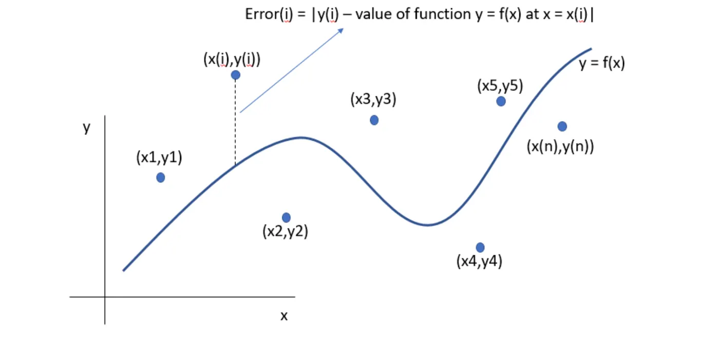
Suppose each of these n points has an individual error (difference in y co-ordinate values)

The error for a general “I” point can be given by the function,

Error= |y(i) – value of f(x) at x(i)| = |y(i)-f(x(i)) |

To remove the modulus sign, it is effective if we square the error term, when we square the error terms and add the errors for all the ‘n’ points we get,

Assume the proposed equation is an nth degree polynomial of the form,

When we differentiate the SSE with every coefficient of the proposed equation f(x) and we equate it to zero, we can find the minima and the value of that coefficient.

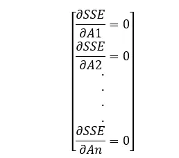
Upon solving the multiple systems of equations, we can find the values of all the coefficients. This method is known as the Least Squares Method and is the most commonly used technique as long as the fitting function is a polynomial.

R-square

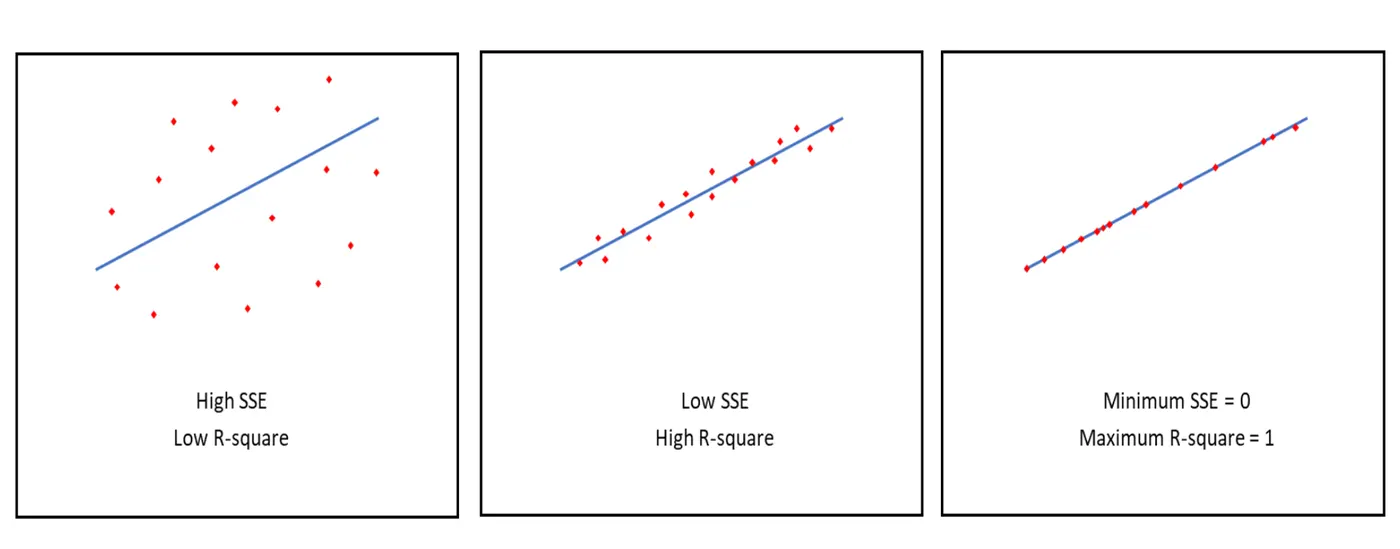
This quantity that measures how successful the fit is in explaining the variation of the data. R-square is the square of the correlation between the response values and the predicted response values. It is also called the square of the multiple correlation coefficient and the coefficient of multiple determination.

The higher the value of R-square the better the fit, the lower it is the lousier the fit, R-square ranges from a value of 0 to 1

0 for the worst possible fit for the data set

1 for the best possible fit for the data set.

The value of R-square can be calculated using the following formula,

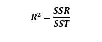
Where,

SSR= sum of squares of the regression, which is the square of the difference between the value of the fitting function at a given point and the arithmetic mean of the data set.

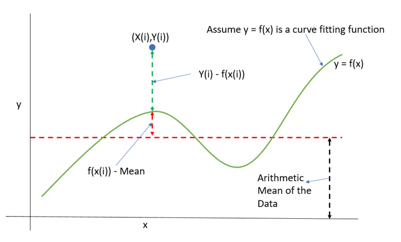
If y=f(x) is the fit curve then the SSR is defined as follows,

SSR=

Similarly, SSE is defined as follows,

SSE=

Now the term SST is given by the summation of SSR and SSE

SST=SSR +SSE

From here, we can calculate the value of R^2,

Adjusted R-Square

It is a normalizing variation of R-square which neglects the variation of R-square due to insignificant independent variables.

For, y=f(x1,x2, x3,…., xn) here x1,x2,x3,…,xn are the independent variables and y is the dependent variable.

If the value of x(i) contributes to the output y then x(i) is a significant dependent variable

If the value of x(i) does not contribute to the output y, then x(i) is an insignificant dependent variable.

This method disregards these infinitesimally small increments to R-square, and only considers the variables which contribute to the output of the system drastically.

R- square is formulated as:

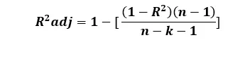
Where,

n- the number of data points

k- the number of independent variables

Here, there can be 2 possibilities

1. The newly added independent variable is significant then R-square will increase greatly. As a result, Adjusted R-square will increase
2. The newly added independent variable is insignificant, R-square will change very less. As a result, Adjusted R-square will increase.

RMSE (Root Mean Square Error)

This static is also known as the fit standard error of the regression. It is an estimate of the standard deviation of the random component in the data and is defined as,

Where,

n is the total number of od data points available.

Treating different types of polynomial equations:

The first-degree polynomial equation

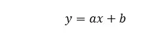
is a line with slope a. A line will connect any two points, so a first-degree polynomial equation is an exact fit through any two points with distinct x coordinates.

If the order of the equation is increased to a second-degree polynomial, the following results:

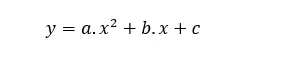
This will exactly fit a simple curve to three points.

If the order of the equation is increased to a third-degree polynomial, the following is obtained:

This will exactly fit four points.

A more general statement would be to say it will exactly fit four constraints. Each constraint can be a point, angle, or curvature (which is the reciprocal of the radius of an osculating circle). Angle and curvature constraints are most often added to the ends of a curve, and in such cases are called end conditions. Identical end conditions are frequently used to ensure a smooth transition between polynomial curves contained within a single spline.

Curve Fitting in Python

Given a Dataset comprising of a group of points, find the best fit representing the Data.

We often have a dataset comprising of data following a general path, but each data has a standard deviation which makes them scattered across the line of best fit. We can get a single line using a curve-fit () function.

Using SciPy:
Scipy is the scientific computing module of Python providing in-built functions on a lot of well-known Mathematical functions. The scipy. optimize package equips us with multiple optimization procedures.

4. Write code to fit a linear and cubic polynomial for the Cp data. Explain if your results are good or bad.

Code:

import math
import matplotlib.pyplot as plt 
import numpy as np 
from scipy.optimize import curve_fit

def func1(t,a,b):
	return a*t + b

def func2(t,a,b,c,d):
	return a*pow(t,3) + b*pow(t,2) + c*t + d

def read_file():
	temperature=[]
	cp=[]
	for line in open('data', 'r'):
		values=line.split(',')
		temperature.append(float(values[0]))
		cp.append(float(values[1]))
	return [temperature, cp]

temperature,cp=read_file()
popt1,pcov1=curve_fit (func1, temperature, cp)
popt2,pcov2=curve_fit (func2, temperature, cp)
fit_cp1=func1(np.array(temperature), *popt1)
fit_cp2=func2(np.array(temperature), *popt2)

plt.figure()
plt.plot(temperature, cp, color='blue', lw=3)
plt.plot(temperature, fit_cp1, color='red', lw=3)
plt.legend(['Actual data', 'Linear cure fit'])
plt.title('Linear curve fit')
plt.xlabel('temperature[k]')
plt.ylabel('cp')
plt.show()

plt.figure()
plt.plot(temperature, cp, color='blue', lw=3)
plt.plot(temperature, fit_cp2, color='green', lw=3)
plt.legend(['Actual data', 'Cubical cure fit'])
plt.title('Cubical curve fit')
plt.xlabel('temperature[k]')
plt.ylabel('cp')
plt.show()

Conclusion:

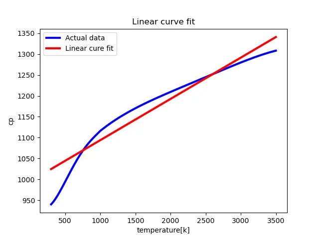
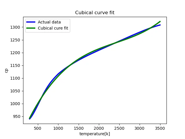
It is clear from the above figures that the curve fits better when the degree of the polynomial increases. It can be observed that the deviation of the curve fit with the actual data is more for linear equation and gradually the deviation decreases with the increase in the order of the polynomial.

5. What needs to be done to make the curve fit perfectly?

Changes to be made to get a better fit:

1. The order of the polynomial should be increased.
2. The given data needs to be divided into parts and then the fit needs to be found.

Another method to get a better fit could be using split wise polynomial.

Discussion:

There are two types of the curve fit Exact and Best. The curve can be made fit perfectly by increasing the order of polynomial or by using non-linear regression. Best fit can de be obtained by the Least Square Regression Method known as L.S.R Cubic fit can be improved by centering and scaling.