Week 5 - Curve fitting

AIM:

To Code to fit a linear and cubic polynomial for the Cp data.

THEORY:

Curve fitting: It is one of the most powerful and most widely used analysis tools in Origin. Curve fitting examines the relationship between one or more predictors (independent variables) and a response variable (dependent variable), with the goal of defining a "best fit" model of the relationship.

Curve fitting with linear and non-linear regression:

In regression analysis, curve fitting is the process of specifying the model that provides the best fit to the specific curves in your dataset. Curved relationships between variables are not as straightforward to fit and interpret as linear relationships.

For linear relationships, as you increase the independent variable by one unit, the mean of the dependent variable always changes by a specific amount. This relationship holds true regardless of where you are in the observation space.

1.With using polynomial terms in linear regression:

The most common method is to include polynomial terms in the linear model. Polynomial terms are independent variables that you raise to a power, such as squared or cubed terms.

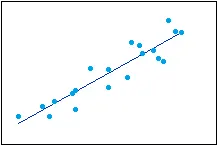
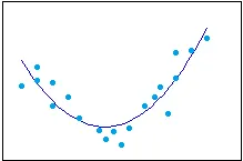
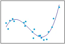
To determine the correct polynomial term to include, simply count the number of bends in the line. Take the number of bends in your curve and add one for the model order that you need.

For Exmaple:

GOODNESS OF FIT:

If you want to know the "goodness of fit", use the R squared stat. R squared tells you how much of the observed variance in the outcome is explained by the input. Here is an example in python.

FOR EXAMPLE:

import numpy as np
from sklearn.linear_model import LinearRegression
import matplotlib.pyplot as plt
from sklearn.metrics import r2_score
#Your data
np.random.seed(0)
N = 1000
x = np.random.normal(size = N)
y = 2*x+1 + np.random.normal(size = N)

#Your model
model=LinearRegression()
model.fit(x.reshape(-1,1),y)

#Your statsitic
r2_score(y, model.predict(x.reshape(-1,1)))

This returns 0.801, so 80.1% per cent of the variance in y seems to be explained by x. The higher this number the better.

As for assessing fit over different regions, I think you can look at the residuals of your model and see if there are patterns or heterogeneity of variance.

Interpretation of R squared:

That is, it measures the variance accounted for by the nonlinear model over and above that which is accounted for
by the mean of Y. When the model does not contain an intercept-type term, this representation of R-Squared must
be used carefully. You should also note that the predicted values, Yi  , might be in the original (untransformed)
metric or in a transformed metric. The program selects what we feel is the appropriate metric in each situation.
A common misconception is a view that R-Squared, the proportion of explained variation, is useful as a
goodness-of-fit index in all nonlinear regression situations. Only when you have a linear model with a constant
term does R-Squared represent the proportion of variation explained

IMPORTANT TERMS:

1.popt: Values of Coefficients of the equation.

2.pcov: The pcov variable contains the covariance matric i.e., it is the estimated covariance of popt.The diagonals provide the variance of the estimate of the coefficient.From them, we can determine the standard deviations of the coefficients

3.np.array(temperature), it does pass values of temperature as arrays.

4. The * in *popt mean that it will expand a list of values into arguments of the function.

5. How to make a curve fit perfectly?

ans: curve fit can be made perfectly by eliminating the errors and it must fit the original curve

errors are like centring and scaling

6. How to get the best fit?

ans: to get the best fit we can go up to higher-order ode or we can use split-wise data method.

note: split wise data method gives us the best fit at lower order

CODE EXPLANATION:

1. First, consider the linear equation and write a code for it to execute.

2. Using open command open the file and read it.

3. append the values in respective variables.

4. Using, popt,pcov=curve_fit(func,temperature,cp) plot the graph and make necessary judgments that curve is fit or not, if otherwise go with higher polynomial until the curve gets fit.

import matplotlib.pyplot as plt
import numpy as np
from scipy.optimize import curve_fit

def func(t,a,b):
	return a*t+b
def read_file():
	temp=[]
	cp=[]
	for line in open('data','r'):
		values=line.split(',')
		temp.append(float(values[0]))
		cp.append(float(values[1]))
	return[temp,cp]

temperature,cp=read_file()

popt,pcov=curve_fit(func,temperature,cp)
print(pcov)
fit_cp=func(np.array(temperature),*popt)

plt.figure()
plt.plot(temperature,cp)
plt.plot(temperature,fit_cp)
plt.savefig('.png')
plt.show()

import matplotlib.pyplot as plt
import numpy as np
from scipy.optimize import curve_fit

def func(t,a,b,c,d):
	return a*pow(t,3)+b*pow(t,2)+c*t+d
def read_file():
	temp=[]
	cp=[]
	for line in open('data','r'):
		values=line.split(',')
		temp.append(float(values[0]))
		cp.append(float(values[1]))
	return[temp,cp]

temperature,cp=read_file()

popt,pcov=curve_fit(func,temperature,cp)
print(pcov)
fit_cp=func(np.array(temperature),*popt)

plt.figure()
plt.plot(temperature,cp)
plt.plot(temperature,fit_cp)
plt.savefig('.png')
plt.show()

import matplotlib.pyplot as plt
import numpy as np
from scipy.optimize import curve_fit

def func(t,a,b,c,d,e):
	return a*pow(t,4)+b*pow(t,3)+c*pow(t,2)+d*pow(t,1)+e
def read_file():
	temp=[]
	cp=[]
	for line in open('data','r'):
		values=line.split(',')
		temp.append(float(values[0]))
		cp.append(float(values[1]))
	return[temp,cp]

temperature,cp=read_file()

popt,pcov=curve_fit(func,temperature,cp)
print(pcov)
fit_cp=func(np.array(temperature),*popt)

plt.figure()
plt.plot(temperature,cp,)
plt.plot(temperature,fit_cp)
plt.savefig('.png')
plt.show()

import matplotlib.pyplot as plt
import numpy as np
from scipy.optimize import curve_fit

def func(t,a,b,c,d,e,f,g,h,i,j):
	return a*pow(t,9)+b*pow(t,8)+c*pow(t,7)+d*pow(t,6)+e*pow(t,5)+f*pow(t,4)+g*pow(t,3)+h*pow(t,2)+i*pow(t,1)+j
def read_file():
	temp=[]
	cp=[]
	for line in open('data','r'):
		values=line.split(',')
		temp.append(float(values[0]))
		cp.append(float(values[1]))
	return[temp,cp]

temperature,cp=read_file()

popt,pcov=curve_fit(func,temperature,cp)
print(pcov)
fit_cp=func(np.array(temperature),*popt)

plt.figure()
plt.plot(temperature,cp)
plt.plot(temperature,fit_cp)
plt.savefig('.png')
plt.show()

OBSERVATIONS:

Here at 9th order polynomial, we are getting exact curve fit.