Week 5.2 - Literature review: ODE Stability

1.

An Ordinary ifferential Equation is an equation containing one or more functions of one independent variable and the derivatives of those functions. Solving them are of paramount importance, as they govern a range of phenomena. One of the key characteristics of the Solution to an Ordinary Diefferntial Equation is Stability. Here, we shall discuss the following methods of solving ODEs :

• Explicit : This uses the value of previous time-step to calculate the value at current time-step.
• Implicit : This method solves the System of Equations to calculate the value at current time-step.

An ODE becomes unstable when it's solution diverges, i.e, small changes in Initial Conditions lead to large changes in Solution. Instability may also happen as a result of Error Amplification. In practice, this usually happens when the step-size is rather large. Implicit Methods are unconditionally stable as they involve solving the parent equation at every step, however, this leads to the requirement of higher computational effort, thus increasing time & cost. When it comes to Explicit Methods though, stability is highly dependent on the step-size. Divergence of the solution as such are problematic as they give unphysical results.

Below, we compare the behaivour of Euler's Implicit & Euler's Explicit Schemes with the Analytical Solution of the given ODE :

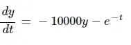
Euler's Explicit Method (Forward Differencing) :

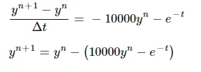
Here, n is the old value.

Euler's Implicit Method (Backward Differencing) :

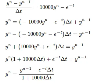
Here, n is the new value.

This is done using the following code :

# This Program compares the results of various Explicit & Implicit Methods (for solving an ODE)
# with the Analytical Solution

"""
We consider the following ODE :

    f_dash(y , t) = dy/dt = -1000y - (e)^(-t)

Explicit :

Euler's Forward Difference Method : 
   (y_(n+1) - y_n) / dt = f_dash(y_n , t_n)        Here, n is the old value
=> y_(n+1) = y_n + f_dash(y_n , t_n)*dt
Stability Value = (1 - 100*dt)
 
Implicit :

Euler's Backward Difference Method : 
   (y_n - y_(n-1))/dt = f_dash(y_n , t_n)          Here, n is the new value
=> y_n = y_(n-1) + f_dash(y_n , t_n)*dt
Stability Value = 1/(1 + 1000*dt)

"""

import numpy as np
import matplotlib.pyplot as plt

t_final = 0.1       # Maximum Time
dt = 0.0001         # Time-Step

# Defining the ODE
def f_dash(t, y) :      
    return (-1000*y) - (np.exp(-t))

# Defining function for Explicit Euler (Forward Difference)  
def explicit_euler(t_final, dt) :
    
    t = np.arange(0, t_final, dt)   # linspace takes in the number of steps as the 3rd parameter,
    y = np.zeros(len(t))            # whereas, arange requires the step-size.
    
    for i in range(1, len(t)) :
        y[i] = y[i-1] + (dt * f_dash(t[i-1], y[i-1]))
    return [t, y]       # a 2-D Array containing values of t & y

# Defining function for Implicit Euler (Backward Difference)
def implicit_euler(t_final, dt) :
    
    t = np.arange(0, t_final, dt)
    y = np.zeros(len(t))
    
    for j in range(1, len(t)) :
        y[j] = (y[j-1] - (dt * np.exp(-t[j]))) / (1 + 1000*dt)
    return [t, y]

# Defining the Analytical Solution
def analytical(t_final, dt) :

    t = np.arange(0, t_final, dt)
    y = np.zeros(len(t))

    for k in range(1, len(t)) :
        y[k] =  (np.exp(-1000*t[k]) * (1 - np.exp(999*t[k])))/999
    return [t, y]

t, y_explicit = explicit_euler(t_final, dt)     
t, y_implicit = implicit_euler(t_final, dt)
t, y_analytical = analytical(t_final, dt)

# Plotting the Results
plt.plot(t, y_implicit, color = 'blue', label = 'Implicit')
plt.plot(t, y_explicit, color = 'red', label = 'Explicit')
plt.plot(t, y_analytical, color = 'black', label = 'Analytical')
plt.legend()
plt.xlabel('t', fontweight = 'bold')
plt.ylabel('y', fontweight = 'bold')
plt.title('dt = 0.0001', fontweight = 'bold')
plt.grid('on')

plt.show()

The results being :

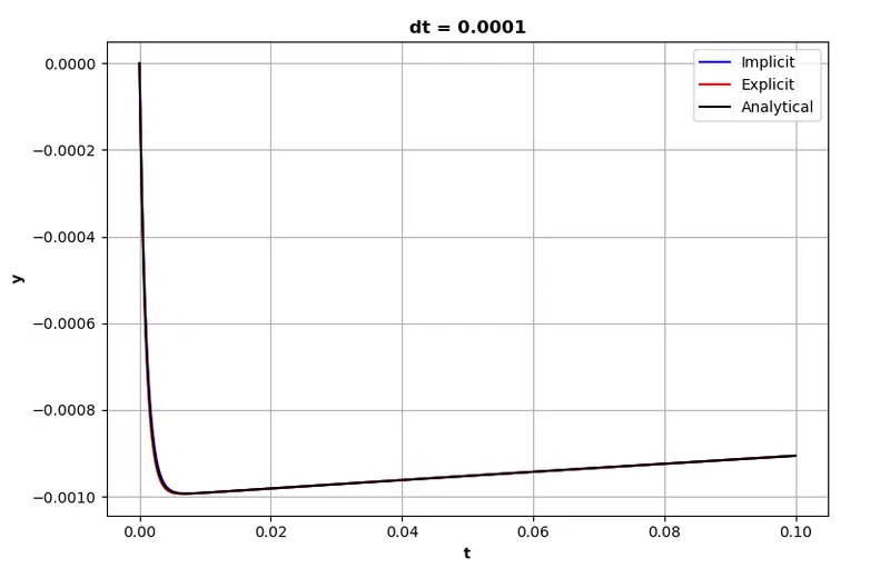
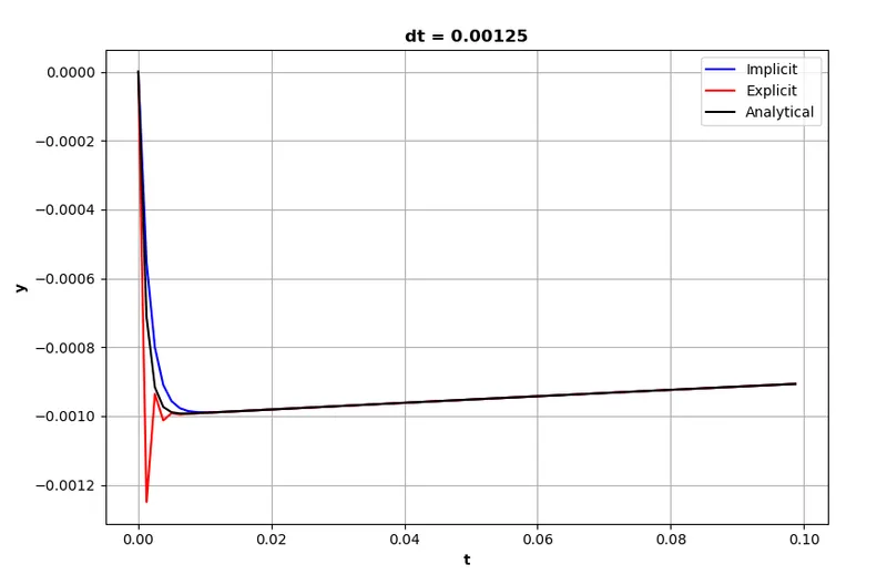
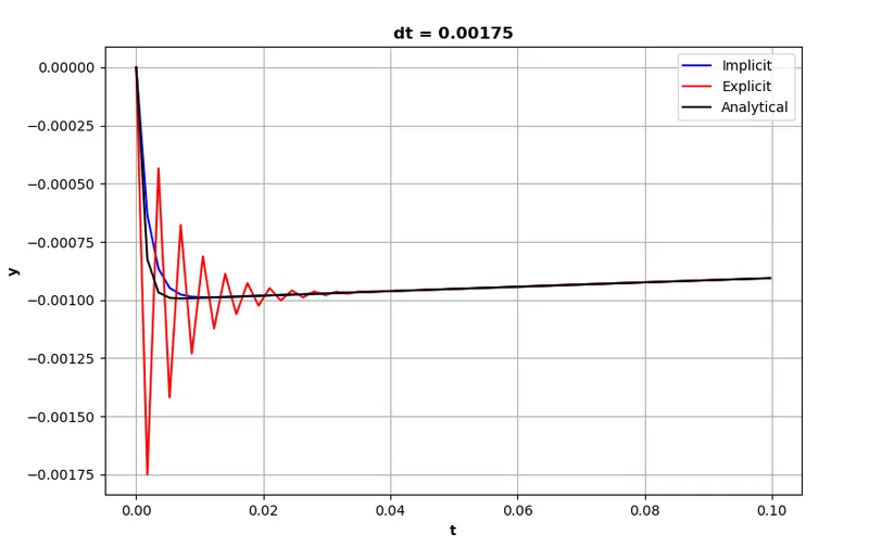
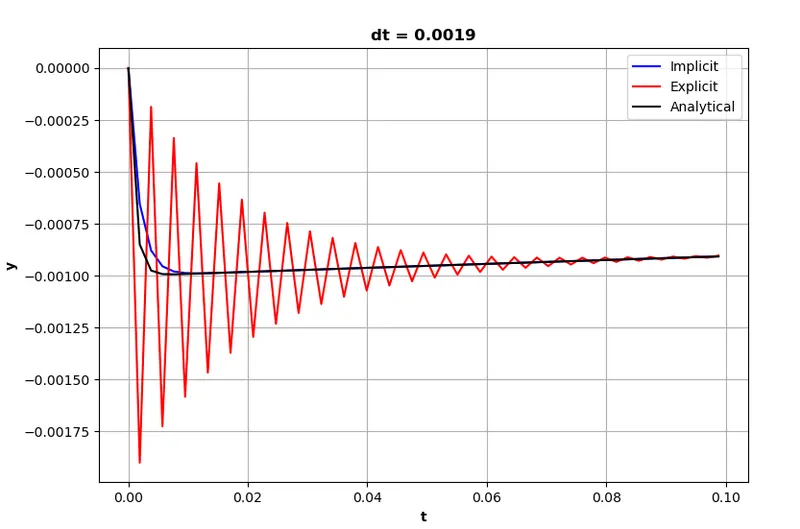
It can be clearly observed that, while Implicit largely agrees with the Analytical Solution, the Explicit Solution is exteremely sensetive to the time-step value. At dt = 0.0001, all the methods agree perfectly, where as staring from dt = 0.00125, the Explicit Solution blows up & it keeps worsening with increasing dt. The stability criteria can be derived for a particular type of problem. Stability of Linear Problems (as the above) depend on the time-step size, which can be controlled to steer the solution towards stability.