Week 5.2 - Literature review: ODE Stability

Introduction:

There are 2 systems in mathematics, stable and unstable systems. In a stable system, a certain small amount of disturbance is inserted into the system, then it tends to minimize it. If the disturbance amplifies as the system progresses in time and does not decrease in value, then it is called an unstable system. The ordinary differential equation is a differential equation containing one or more functions of one independent variable and the derivatives of those functions.

Euler method:-

In mathematics and computational science, the Euler method is a first-order numerical procedure for solving ordinary differential equations with a given initial value. It is the most basic explicit method for numerical integration of ordinary differential equations and is the simplest Runge–Kutta method.

In Euler's method, we used a technique used to analyze a Differential Equation, which uses the idea of linear approximation, where we use small tangent lines over a short distance to approximate the solution to an initial-value problem.

The expression that can be derived from the process is:

`y_(i+1) = y_i + h*f(t_i,y_i)`

where h is the length of the sub interval and `y_i`is an approximation of the solution to the ODE at a time `t_i`. Now, Euler's method is the explicit scheme.

However, the above expression is stable only for small values of h. When the length of the sub interval(h) increases, the error also increases, then the system becomes unstable.

To overcome this drawback, Euler's method is modified a little. The modified Euler's method is known as an implicit scheme.

`y_(i+1) = y_i + h*f(x_(i+1),y_(i+1))` here `y_(i+1)` is appearing in both sides, so it is implicit.

The stability criteria can be understood by using a general single-step method equation.

`y_(i+1) = E*y_i`

For absolute stability, `abs(E) <= 1`.

1) The ODE becomes unstable only for large time steps in the explicit method.

The differential equation for the explicit method: `dy/dx = -1000*y-e^-x`.

Code:

'''
	Explicit eular demo 
'''
import matplotlib.pyplot as plt 
import math

def f(t,y):
	return -1000*y-math.exp(-t)

t_start = 0
t_end = 0.1
n = 500

dt = (t_end - t_start)/(n-1)

t = 0
y_old = 0
y_new = []
for i in range(0,n):
	y_new.append(y_old + dt*f(t,y_old))
	t = t+dt
	y_old = y_new[i]
	print(y_new)

plt.plot(y_new)
plt.show()

Result:

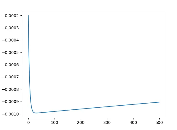
For figure:1, n = 500 and t_end = 0.1. In this figure the solution is stable.

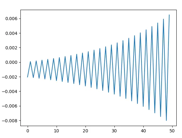
For figure:2, n = 50 and t_end = 0.1. In this figure the solution is unstable.

2) How does stability affect engineering simulations?

Stability plays an important role in engineering simulations. If a solution becomes unstable, the required value will deviate instead of converging. Due to this error, we didn't get a perfect output for engineering simulations.

3) Can stability conditions be derived for all types of problems?

Yes, stability conditions be derived for all types of problems and it depends upon the nature of the function. Eigenvalue stability condition and Von Neumann stability condition are the most common stability conditions.