Week 5.2 - Literature review: ODE Stability

1. When does a ODE become unstable?

To answer this question it is essential to undertsand the type of numerical schemes available to solve and ODE. Solving an ODE analytically could be tedious. However, numerical methods for ODE prove to be efficient while dealing with more than one parameters. The numerical approximation/computation of integrals, know as Runge-Kutta methods are done in temporal discretization.

• Forward Euler method (is an explicit scheme): Explicit Runge–Kutta methods are generally unsuitable for the solution of stiff equations because their region of absolute stability is small; in particular, it is bounded.

y(n+1)=y(n)+f(t(n),y(n))dt

• Backward Euler method (is an implicit scheme) :The instability of explicit Runge–Kutta methods motivates the development of implicit methods.

y(n+1)=y(n)+f(t(n),y(n+1))dt

The error step is proportional to step size and global error at the given time.

For example let's understand the behavior of the following equation with change in timestep.

f(y)=-1000y-e^-t

__code:______________________________________________________________________________

import math
import matplotlib.pyplot as plt
import numpy as np

def explicit(t_total,dt):
t=np.arange(0,t_total,dt)
y=np.zeros(len(t))

for i in range(0,len(t)):
y[i]=y[i-1]+dt*(-1000*y[i-1]-np.exp(-t[i-1]))
return[t,y]

def implicit(t_total,dt):
t=np.arange(0,t_total,dt)
y=np.zeros(len(t))

for i in range(0,len(t)):
y[i]= (y[i-1]-np.exp(-t[i])*dt)/ (1+1000*dt)
return[t,y]

def analy(t_total,dt):
t=np.arange(0,t_total,dt)
y=np.zeros(len(t))

for i in range(0,len(t)):
y[i]=np.exp(-1000*t[i])*(1-np.exp(999*t[i]))/999
return[t,y]

t_total =1
dt=1e-4 #Changing this will affect the stability of the solution

t,y_exp=explicit(t_total,dt)
t,y_imp=implicit(t_total,dt)
t,y_analy=analy(t_total,dt)

plt.plot(t,y_exp,color='red')
plt.plot(t,y_imp,color='blue')
plt.plot(t,y_analy,color='green')

plt.legend(["Explicit","Implicit","Analytical"])
plt.grid('on')
Heading=('Timestep"',dt)
plt.title(Heading)
plt.show()

________________________________________________________________________________

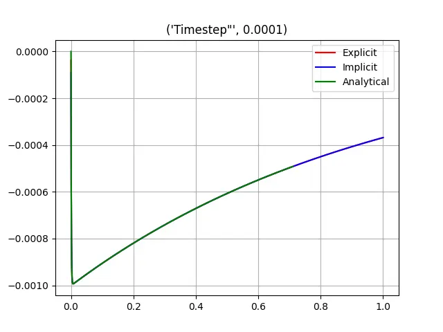
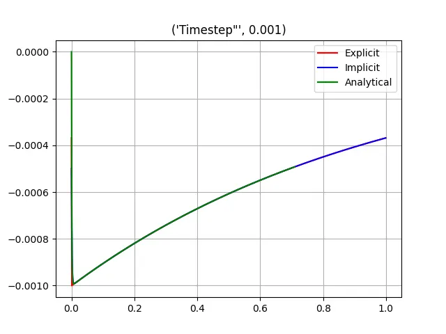
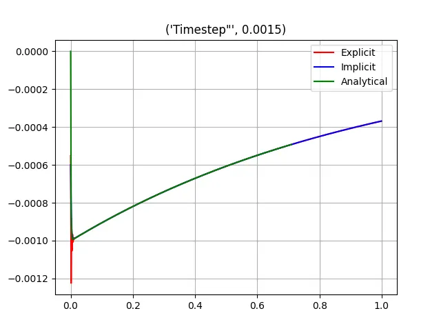
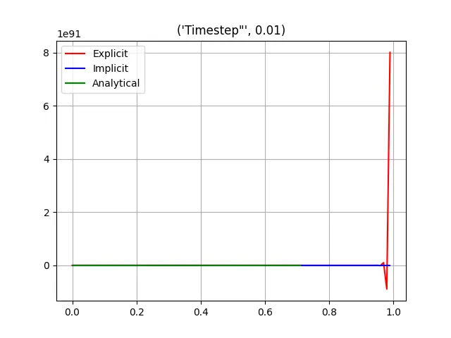
The smallest value of dt provides a stable solution. But as the dt value increae teh explicit solution grows increasingly unstable, however, the implicit scheme is in good adherance with the analytical solution. Therefore, the implicit scheme is prefered for solving ODE.

2.How does stability affect engineering simulations?

Any solution is expected to reach an equilibrium after a certain point to be useful as a relaible solution to the engineering problem/model etc. Unstable solutions oscillate largely and never reach a stable point. In physical sense a oscillating solution is far away from a mathematical value that accurately defines the state of the system at that given time. Smaller the step size smaller the error.

3. Can stability condition be derived for all types of problems?

No, stability condition can be derived for linear ODEs using state transition matrix. For non-linear ODE, a jacobian matrix is defined comprising of the first order derivative of the of all teh functions w.r.t the independent variables. If all the eigen values calculated from this matrix are negetive, the system is stable else not.