Week 5.1 - Mid term project - Solving the steady and unsteady 2D heat conduction problem

AIM:
To solve 2D heat conduction equation for steady and transient state using various iterative techniques such as Jacobi, Gauss Seidel and Successive over relaxation methods using MATLAB.

Steady-state analysis:
The 2D Transient equation: 𝑑𝑇𝑑𝑡∝(𝑑2𝑇𝑑𝑥2+𝑑2𝑇𝑑𝑦2)=0
The Steady-state equation: (𝑑2𝑇𝑑𝑥2+𝑑2𝑇𝑑𝑦2)=0
Assume that the domain is a unit square.
Now assigning boundary conditions.
Temperatures for steady-state
T_L=400; %Temp at left boundary
T_T=600; %Temp at top boundary
T_R=800; %Temp at right boundary
T_B=900; %Temp at bottom boundary
From the above Boundary conditions, we can calculate the central temperature of the domain

(𝑇𝑃)=1/𝐾∙((𝑇𝐿 𝑇𝑅/𝑑𝑥2)+(𝑇𝑇+𝑇𝐵/𝑑𝑦2))

For 2D heat conduction equation we are using the following method:

• JACOBI-In this method, the 2D heat conduction equation solves using calculating the value of temperature at inner nodes using several iterations, in which each values of temperature will be previously assigned temperature values at nodes.
• GAUSS-SEIDEL-In this method, the 2D heat conduction equation solves, we are calculating the value of temperatures at inner nodes using several iterations, in which every value of temperature will be updated successively with respect to the previous iteration.
• SUCCESSIVE OVER-RELAXATION-In this method, the 2D heat conduction equation solves. We are calculating the value of temperatures at inner nodes using several iterations, in which respect to the previous iteration And also “Relaxation factor” multiplies to the algebraic equation to alter the path of the iteration.

When RF<1 under relax
When RF<1 over relax
The Value of Relaxation factor can be taken as 1.1 or 1.2
The Relaxation factor plays a vital role in determining the rate of convergence for CFD simulation

MATLAB Coding for Steady state equation:

clear all
close all
clc
%COd to solve second order 2-dimensional heat conduction equation
%Steady-state Analysis : d^2t/dx^2+d^2/dy^2=0
%Inputs
L=1;
%The domain is a unit square
nx=10;
ny=nx;
%grid points along x and y direction
dx=L/(nx-1);
%Change of x wrt x co-ordinate
dy=L/(ny-1);
%change of y wrt y co_ordinate
x=linspace(0,1,nx);
y=linspace(0,1,ny);
%assigning boundry conditions
% temperatures for stedy and transient case
T_L=400;
T_T=600;
T_R=800;
T_B=900;
T=ones(nx,ny); %temperature array
%updating value of temperatures
T(:,1)=T_L;
T(:,end)=T_R;
T(1,:)=T_T;
T(end,:)=T_B;
3
Told=T;
[x y]=meshgrid(x,y);
%w=2*((dx^2+dy^2)/(dx^2*dy^2));
iterative_solver=1;
error=9e9;
tol=1e-4;
%tolerance value
%jacobi method
tic;
jacobi_iter=1;
while(error>tol)
for i=2:nx-1
for j=2:ny-1
T(i,j)=0.25*((Told(i-1,j)+Told(i+1,j)))+0.25*((Told(i,j-1)+Told(i,j+1)));
end
end
error=max(max(abs(Told-T)));
Told=T;
jacobi_iter=jacobi_iter+1;
end
A=toc;
figure(1)
contourf(x,y,T, 'ShowText','on');
colormap(jet);
colorbar;
title_text=sprintf('JACOBI, Iteration number=%d, computation time=%f', jacobi_iter, A);
title(title_text);
xlabel('X-axis');
ylabel('Y-axis');
set(gca,'YDIR','reverse')
pause(0.003);
%GS method
%Inputs
L=1;
%The domain is a unit square
nx=10;
ny=nx;
%grid points along x and y direction
dx=L/(nx-1);
%Change of x wrt x co-ordinate
dy=L/(ny-1);
%change of y wrt y co_ordinate
x=linspace(0,1,nx);
y=linspace(0,1,ny);
%assigning boundry conditions
% temperatures for stedy and transient case
T_L=400;
T_T=600;
T_R=800;
T_B=900;
4
T=ones(nx,ny);
%temperature array
%updating value of temperatures
T(:,1)=T_L;
T(:,end)=T_R;
T(1,:)=T_T;
T(end,:)=T_B;
Told=T;
[x y]=meshgrid(x,y);
%w=2*((dx^2+dy^2)/(dx^2*dy^2));
iterative_solver=1;
error=9e9;
tol=1e-4;
%tolerance value
tic;
gs_iter=1;
while(error>tol)
for i=2:nx-1
for j=2:ny-1
T(i,j)=0.25*((T(i-1,j)+Told(i+1,j)))+0.25*((T(i,j-1)+Told(i,j+1)));
end
end
error=max(max(abs(Told-T)));
Told=T;
gs_iter=gs_iter+1;
end
B=toc;
figure(2)
contourf(x,y,T, 'ShowText','on');
colormap(jet);
colorbar;
title_text=sprintf('GS, Iteration number=%d, computation time=%f', gs_iter, B);
title(title_text);
xlabel('X-axis');
ylabel('Y-axis');
set(gca,'YDIR','reverse')
pause(0.003);
% Successive over relaxation method
%Inputs
L=1;
%The domain is a unit square
nx=10;
ny=nx;
%grid points along x and y direction
dx=L/(nx-1);
%Change of x wrt x co-ordinate
dy=L/(ny-1);
%change of y wrt y co_ordinate
x=linspace(0,1,nx);
y=linspace(0,1,ny);
5
%assigning boundry conditions
% temperatures for stedy and transient case
T_L=400;
T_T=600;
T_R=800;
T_B=900;
T=ones(nx,ny);
%temperature array
%updating value of temperatures
T(:,1)=T_L;
T(:,end)=T_R;
T(1,:)=T_T;
T(end,:)=T_B;
Told=T;
[x y]=meshgrid(x,y);
%w=2*((dx^2+dy^2)/(dx^2*dy^2));
iterative_solver=1;
error=9e9;
tol=1e-4;
%tolerance value
%jacobi method
tic;
sor_iter=1;
omega=1.1
%relaxation factor
while(error>tol)
for i=2:nx-1
for j=2:ny-1
T(i,j)= (1-omega)*Told(i,j)+omega*(0.25*((T(i-1,j)+Told(i+1,j)))+0.25*((T(i,j-1)+Told(i,j+1))));
end
end
error=max(max(abs(Told-T)));
Told=T;
sor_iter=sor_iter+1;
end
C=toc;
figure(3)
contourf(x,y,T, 'ShowText','on');
colormap(jet);
colorbar;
title_text=sprintf('SOR, Iteration number=%d, computation time=%f', sor_iter, A);
title(title_text);
xlabel('X-axis');
ylabel('Y-axis');
set(gca,'YDIR','reverse')
pause(0.003);

Temperature plots:
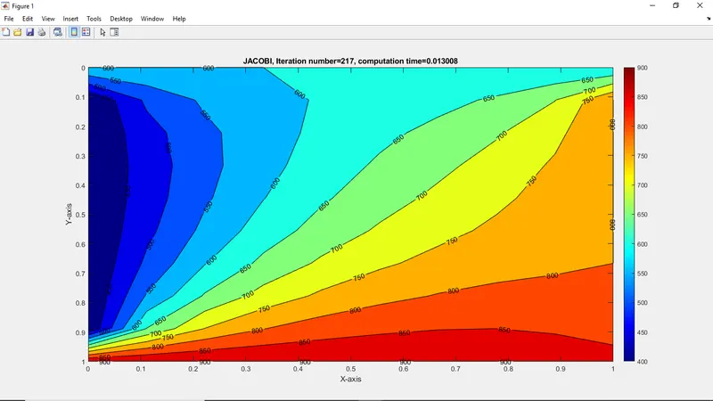
Jacobi method:

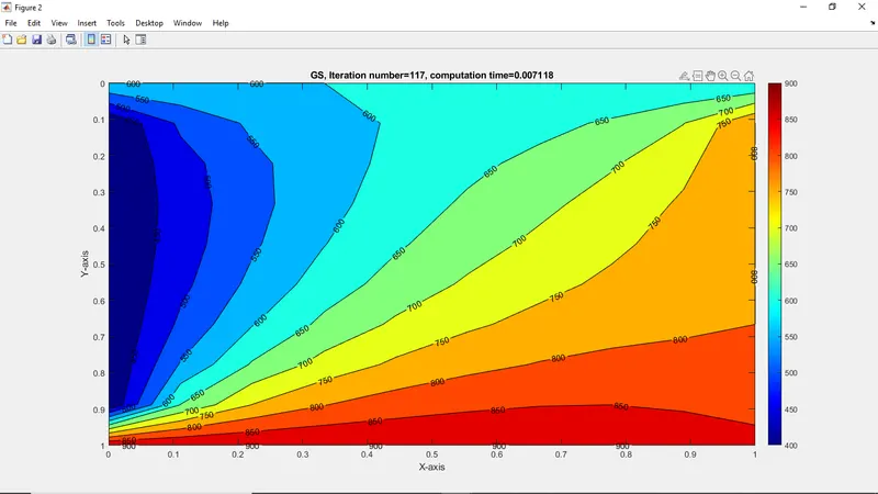
Gauss-seidel method:

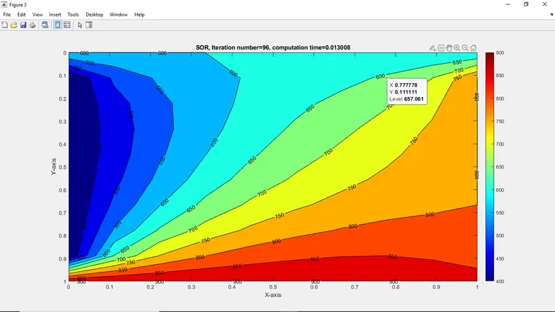
Successive Over Relaxation method:

STEADY STATE RESULTS:

Method Iteration No Computation time
Jacobi 217 0.013008
Gauss-seidel 117 0.007118
Successive-over 96 0.013008
Relaxation

Transient thermal analysis:

Transient thermal analysis is the analysis of the change in properties of the substance that occur due to change in temperature calculated over a particular period of time.
The 2D Transient equation: 𝑑 𝑇/𝑑𝑡 ∝(𝑑^2 𝑇/𝑑𝑥^2+d^2 𝑇/𝑑y^2)=0
For explicit method

Difference equation ad Re-arranging:

𝑇𝑃(𝑛+1)=𝑇𝑃(𝑛)+𝐾1∙(𝑇𝐿 −2∙𝑇𝑃+𝑇𝑅)(𝑛)+𝐾2∙(𝑇𝑇−2∙𝑇𝑃+𝑇𝐵)(𝑛)
Where K1 &K2 are CFL values in x and y direction.
𝐾1=𝛼∙𝑑𝑡/𝑑𝑥2 ; 𝐾2=(𝛼∙𝑑𝑡)∙𝑑𝑦2
For explicit term the CFL value should <=0.5 to make the solution stable.

MATLAB Coding for Explicit method:

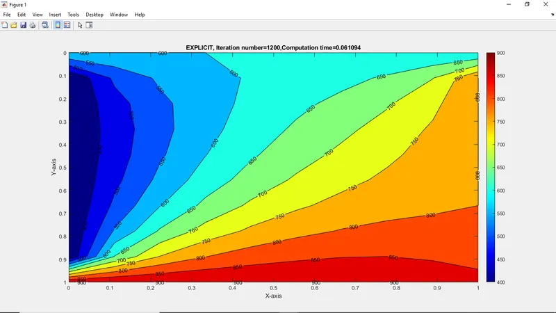
clear all
close all
clc
%COd to solve second order 2-dimensional heat conduction equation_EXPLICIT_METHOD
%unSteady-state Analysis : (dT/dt)-alphad^2T/dx^2+d^2/dy^2=0
%Inputs
L=1;%The domain is a unit square
nx=10;
ny=nx; %grid points along x and y direction
dx=L/(nx-1); %Change of x wrt x co-ordinate
dy=L/(ny-1); %change of y wrt y co_ordinate
alpha=1.4; %heat conduction coeficient
dt=1e-3; %time step
t=1.2; %time initialization
nt=t/dt; %no of timesteps
x=linspace(0,1,nx);
y=linspace(0,1,ny);
%assigining boundary conditions
%temperatures for steady and transient case
T_L=400; %Temp at left boundary
T_T=600; %Temp at top boundary
T_R=800; %Temp at right boundary
T_B=900; %Temp at bottom boundary
T=ones(nx,ny); %temperature array
%updating values of temperatures
T(:,1)=T_L;
T(:,end)=T_R;
T(1,:)=T_T;
T(end,:)=T_B;
Told=T;
[x y]=meshgrid(x,y);
%w=2*((dx^2+dy^2)/(dx^2*dy^2));
%
9
% iterative_solver=1;
% error=9e9;
% tol=1e-4; %tolerance value
alpha=1.4; %heat transfer coeficient
%CFL numbers
k1=(alpha*dt)/dx^2;
k2=(alpha*dt)/dy^2;
%explicit methods
tic;
% explicit_iter=1;
% while(error>tol)
for k=1:nt
for i=2:nx-1
for j=2:ny-1
T(i,j)=Told(i,j)+k1*(Told(i-1,j)-2*Told(i,j)+Told(i+1,j))+k2*(Told(i,j-1)-2*Told(i,j)+Told(i,j+1));
end
end
error=max(abs(Told-T));
Told=T;
% explicit_iter=explicit_iter+1;
end
time=toc;
figure(1)
contourf(x,y,T,'ShowText','on');
colormap(jet)
colorbar;
title_text=sprintf('EXPLICIT, Iteration number=%d,Computation time=%f',nt,time);
title(title_text);
xlabel('X-axis');
ylabel('Y-axis');
set(gca,'YDIR','reverse')
pause(0.003);

Plot:

Difference equation for implicit scheme:

𝑇𝑃(𝑛+1)=𝑇𝑃(𝑛+1)+𝐾1∙(𝑇𝐿 −2∙𝑇𝑃+𝑇𝑅)(𝑛+1)+𝐾2∙(𝑇𝑇−2∙𝑇𝑃+𝑇𝐵)(𝑛+1)

MATLAB Coding Implicit Method:

clear all
close all
clc
%COd to solve second order 2-dimensional heat conduction equation_IMPLICIT_METHOD
%unSteady-state Analysis : (dT/dt)-alphad^2T/dx^2/dy^2=0
%Inputs
L=1;%The domain is a unit square
nx=10;
ny=nx; %grid points along x and y direction
dx=L/(nx-1); %Change of x wrt x co-ordinate
dy=L/(ny-1); %change of y wrt y co_ordinate
alpha=1.4; %heat conduction coeficient
dt=10; %time step
t=1000; %time initialization
nt=t/dt; %no of timesteps
alpha=1.4; %heat transfer coeficient
CFL=(alpha*dt)/dx^2;
x=linspace(0,1,nx);
y=linspace(0,1,ny);
%assigining boundary conditions
%temperatures for steady and transient case
11
T_L=400; %Temp at left boundary
T_T=600; %Temp at top boundary
T_R=800; %Temp at right boundary
T_B=900; %Temp at bottom boundary
T=ones(nx,ny); %temperature array
%updating value of temperatures
T(:,1)=T_L;
T(:,end)=T_R;
T(1,:)=T_T;
T(end,:)=T_B;
Told=T;
T_previous=T;
[x y]=meshgrid(x,y);
%w=2*((dx^2+dy^2)/(dx^2*dy^2));
% iterative_solver=1;
error=9e9;
tol=1e-4;
%CFL numbers
k1=(alpha*dt)/dx^2;
k2=(alpha*dt)/dy^2;
% assigining the terms
term1=(1+2*k1+2*k2)^-1;
term2=k1*term1;
term3=k2*term1;
prompt= 'Choose solver 1 = jacobi, 2 = GS, 3 = SORn';
method = input(prompt);
%Jacobi methods
tic;
if method==1
jacobi_iter=1;
% error=9e9;
%
% tol=1e-4;
for k=1:nt
while(error>tol)
for i=2:nx-1
for j=2:ny-1
H=(Told(i-1,j)+Told(i+1,j));
V=(Told(i,j-1)+Told(i,j+1));
T(i,j)=(term1*T_previous(i,j))+(term2*H)+(term3*V);
end
end
error=max(max(abs(Told-T)));
Told=T;
jacobi_iter=jacobi_iter+1;
12
end
T_previous=T;
end
time=toc;
figure(1)
contourf(x,y,T, 'ShowText','on');
colormap(jet);
colorbar;
title_text=sprintf('JACOBI, Iteration number=%d, computation time=%f, CFL=%f', jacobi_iter,time,CFL);
title(title_text);
xlabel('X-axis');
ylabel('Y-axis');
set (gca,'YDIR','reverse')
pause(0.003);
end
%GS methods
if method==2
tic;
gs_iter=1;
for k=1:nt
while(error>tol)
for i=2:nx-1
for j=2:ny-1
H=(T(i-1,j)+Told(i+1,j));
V=(T(i,j-1)+Told(i,j+1));
T(i,j)=(term1*T_previous(i,j))+(term2*H)+(term3*V);
end
end
error=max(max(abs(Told-T)));
Told=T;
gs_iter=gs_iter+1;
end
T_previous=T;
end
time=toc;
figure(2)
contourf(x,y,T, 'ShowText','on');
colormap(jet);
colorbar;
title_text=sprintf('GAUSS-SEIDEL, Iteration number=%d, computation time=%f, CFL=%f', gs_iter,time,CFL);
13
title(title_text);
xlabel('X-axis');
ylabel('Y-axis');
set (gca,'YDIR','reverse')
pause(0.003);
end
%Successive over relaxation methods
if method==3
tic;
omega=1.4; %relaxation factor
sor_iter=1
for k=1:nt
while(error>tol)
for i=2:nx-1
for j=2:ny-1
H=(T(i-1,j)+Told(i+1,j));
V=(T(i,j-1)+Told(i,j+1));
T(i,j)=((1-omega)*Told(i,j))+(omega*((term1*T_previous(i,j)+(term2*H)+(term3*V))));
end
end
error=max(max(abs(Told-T)));
Told=T;
sor_iter=sor_iter+1;
end
T_previous=T;
end
time=toc;
figure(3)
contourf(x,y,T, 'ShowText','on');
colormap(jet);
colorbar;
title_text=sprintf('SOR, Iteration number=%d, computation time=%f, CFL=%f', sor_iter,time,CFL);
title(title_text);
xlabel('X-axis');
ylabel('Y-axis');
set(gca,'YDIR','reverse')
pause(0.003);
end

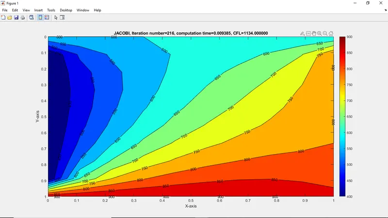
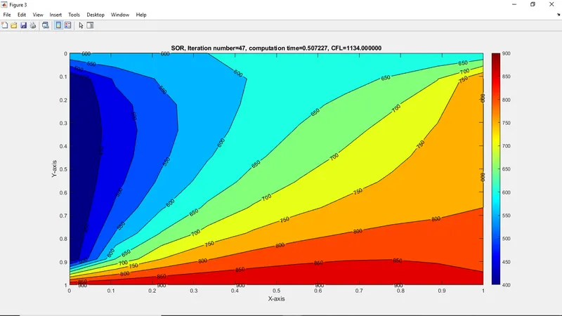
PLOTS:
Jacobi Method:

Gauss Seidel methods: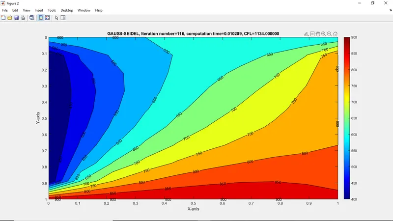

Successive over relaxation methods:

Unsteady state results:
TRANSIENT STATE RESULTS:
Method Iteration NO Computation time
Jacobi 216 0.009385
Gauss-seidel 116 0.010209
Successive-over 47 0.507227
Relaxation

Inference from the Explicit and Implicit Graph:
Explicit Approach:
Relatively simple to program. However, for a given value of dx, dt must be very less than some limit imposed by stability constraints. Hence the CFL no along x and y direction should be less than 0.5 to get stable solutions.

Implicit Approach:
Stability can be maintained over a larger value of dt, hence CFL can be larger, which does not affect the solutions, hence using considerable fever time steps to make calculations for a given interval of t. this results in less computer time. However, it is more complicated to program.

Since large dt can be taken, the truncation error is large, and the use of implicit methods to follow the exact transients (time variation of the independent variable) may not be as accurate as an explicit approach.
However, for a time-dependent solution in which the steady-state is the desired solutions, this relative time wise inaccuracy is not important.

link:

https://documentcloud.adobe.com/link/review?uri=urn:aaid:scds:US:c3ef9f57-eaf4-4d4c-b4df-594c6e062850