Week 5.1 - Mid term project - Solving the steady and unsteady 2D heat conduction problem
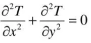
2D Heat Conduction Equation – this the simple equation which represent heat propagation in two dimensions. Steady state 2D heat conduction equation can be written as follows, with assuming no internal heat generation –
Transient state 2D heat conduction equation can be given as follows –
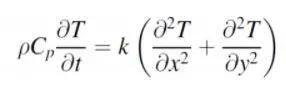
In this study we are going to solve these equations to temperature at a particular node. We will define domain, which will have fixed number of nodes. To find temperature values at nodes, we will use finite difference method. In finite difference method node represents the temperature of a point on the surface being considered. The temperature at node represents the average temperature of that region of the surface. Algebraic equations are used to define the relationship between adjacent nodes on the surface. Increasing number of nodes would lead solution to get high accuracy. After getting equations from finite difference method, the equations will be solved using iterative methods which are Jacobi, Gauss-Seidel and Successive over relaxation (SOR).
Jacobi method – It is simplest iterative method, but comes with more problems than other methods. This method uses predefined values of variable to find new values for each iteration, with a permissible error.
Gauss-Seidel – it is modified Jacobi method, this method uses new values of variable, which is being updated in every iteration.
Successive over relaxation (SOR) – this method is again modified Jacobi, which uses a relaxation factor to new values of variable.
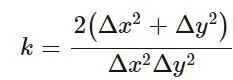
Solution of steady state 2D heat conduction equation is given by following expression –

Solution of transient state 2D heat conduction equation is given by following expression -
Explicit -

Implicit -

MATLAB code –
Steady State -
clear all
close all
clc

% Defining domain
nx = 10;
ny = nx;
% assigning temperature values on the specific nodes and boundaries
t = 250*ones(nx,ny);
told = t;
t(1,1) = 500;
t(length(t),length(t)) = 850;
t(1,length(t)) = 700;
t(1,2:length(t)-1) = 600;
t(length(t),2:length(t)-1) = 900;
t(2:length(t),1) = 400;
t(2:length(t)-1,length(t)) = 800;
t(length(t),1) = 650;
% defining nodes position in domain
x = linspace(0,1,nx);
y = linspace(0,1,ny);
% grid spacing
dx = x(2)-x(1);
dy = dx;
% variable
k = 2*(dx^2+dy^2)/((dx^2)*(dy^2));
% taking input - method type
method =input('Type method number 1-for Jacobi method, 2-for gauss seidel, 3-SOR ');
%relaxation factor
omega = 1.5;
% maximum error
error = 9e9;
% tolerance
tol = 1e-4;

% convergence loop
% jacobi
if method ==1
     iterations = 1;
  while(error>tol)
    for i = 2:nx-1
        for j = 2:ny-1
            t(i,j) = (1/k)*(((told(i-1,j) + told(i+1,j))/dx^2)+((told(i,j-1) + told(i,j+1))/dy^2));
        end
    end
    error = max(max(abs(told -t)));
    told = t;
    iterations = iterations +1;
    contourf(x,y,t,'showtext','on')
    colormap(jet)
    xlabel('x axis')
    ylabel('y axis')
    title(['iterations=',num2str(iterations)])
  end
end

% gauss seidel method
if method ==2
     iterations = 1;
  while(error>tol)
    for i = 2:nx-1
        for j = 2:ny-1
            t(i,j) = (1/k)*(((t(i-1,j) + told(i+1,j))/dx^2)+((t(i,j-1) + told(i,j+1))/dy^2));
        end
    end
    error = max(max(abs(told -t)));
    told = t;
    iterations = iterations +1;
    contourf(x,y,t,'showtext','on')
    colormap(jet)
    xlabel('x axis')
    ylabel('y axis')
    title(['iterations=',num2str(iterations)])
   end
 end

% successive over relaxation
if method ==3
     iterations = 1;
  while(error>tol)
    for i = 2:nx-1
        for j = 2:ny-1
            t_n = (1/k)*(((t(i-1,j) + told(i+1,j))/dx^2)+((t(i,j-1) + told(i,j+1))/dy^2));
            t(i,j) = (1-omega)*t(i,j) + omega*(t_n);
        end
    end
    error = max(max(abs(told -t)));
    told = t;
    iterations = iterations +1;
    contourf(x,y,t,'showtext','on')
    colormap(jet)
    xlabel('x axis')
    ylabel('y axis')
    title(['iterations=',num2str(iterations)])
  end
end
Transient State -
Implicit -
clear all
close all
clc

% Defining domain
nx = 10;
ny = nx;
% assigning temperature values on the specific nodes and boundaries
t = 250*ones(nx,ny);
t(1,1) = 500;
t(length(t),length(t)) = 850;
t(1,length(t)) = 700;
t(1,2:length(t)-1) = 600;
t(length(t),2:length(t)-1) = 900;
t(2:length(t),1) = 400;
t(2:length(t)-1,length(t)) = 800;
t(length(t),1) = 650;
told = t;
t_p = t;
% defining nodes position in domain
x = linspace(0,1,nx);
y = linspace(0,1,ny);
% grid spacing
dx = x(2)-x(1);
dy = dx;
% taking input - method type
method =input('Type method number 1-for Jacobi method, 2-for gauss seidel, 3-SOR ');
%relaxation factor
omega = 1.1;
% maximum error
error = 9e9;
% tolerance
tol = 1e-4;
% time step size
dt = 0.01;
% simulation time
st = 0.4;
% number of time steps
nt = st/dt;
% thermal diffusivity
alpha = 1.2;
% cfl number
k1 = alpha*dt/(dx^2);
k2 = alpha*dt/(dy^2);

% jacobi method
if method ==1
      iterations = 1;
  while(error>tol)
      % time loop
 for k = 1:nt
     % space loop
    for i = 2:nx-1
        for j = 2:ny-1
            term1 = (1+2*k1+2*k2)^-1;
            term2 = k1*term1;
            term3 = k2*term1;
            H = (told(i-1,j)+told(i+1,j));
            V = (told(i,j-1)+told(i,j+1));
            t(i,j) = t_p(i,j)*term1 +H*term2 + V*term3;
        end
    end
    error =max(max(abs(told -t)));
    told = t;
    t_p = t;
    iterations = iterations+1;
    contourf(x,y,t,'showtext','on')
    colormap(jet)
    xlabel('x axis')
    ylabel('y axis')
    title(['iterations=',num2str(iterations)])
 end
  end
end

%Gauss siedel method
if method ==2
      iterations = 1;
  while(error>tol)
 for k = 1:nt
    for i = 2:nx-1
        for j = 2:ny-1
            term1 = (1+2*k1+2*k2)^-1;
            term2 = k1*term1;
            term3 = k2*term1;
            H = (t(i-1,j)+t(i+1,j));
            V = (t(i,j-1)+t(i,j+1));
            t(i,j) = t_p(i,j)*term1 +H*term2 + V*term3;
        end
    end
    error =max(max(abs(told -t)));
    told = t;
    t_p = t;
    iterations = iterations+1;
    contourf(x,y,t,'showtext','on')
    colormap(jet)
    xlabel('x axis')
    ylabel('y axis')
    title(['iterations=',num2str(iterations)])
 end
  end
end

% sor method
if method ==3
      iterations = 1;
  while(error>tol)
 for k = 1:nt
    for i = 2:nx-1
        for j = 2:ny-1
            term1 = (1+2*k1+2*k2)^-1;
            term2 = k1*term1;
            term3 = k2*term1;
            H = (told(i-1,j)+told(i+1,j));
            V = (told(i,j-1)+told(i,j+1));
            t_n = t_p(i,j)*term1 +H*term2 + V*term3;
            t(i,j) = (1-omega)*told(i,j) + omega*t_n;
        end
    end
    error =max(max(abs(told -t)));
    told = t;
    t_p = t;
    iterations = iterations+1;
    contourf(x,y,t,'showtext','on')
    colormap(jet)
    xlabel('x axis')
    ylabel('y axis')
    title(['iterations=',num2str(iterations)])
 end
  end
end
Explicit -
clear all
close all
clc

% Defining domain
nx = 10;
ny = nx;
% assigning temperature values on the specific nodes and boundaries
t = 250*ones(nx,ny);
t(1,1) = 500;
t(length(t),length(t)) = 850;
t(1,length(t)) = 700;
t(1,2:length(t)-1) = 600;
t(length(t),2:length(t)-1) = 900;
t(2:length(t),1) = 400;
t(2:length(t)-1,length(t)) = 800;
t(length(t),1) = 650;told = t;
% defining domain length
x = linspace(0,1,nx);
y = linspace(0,1,ny);
% grid spacing
dx = x(2)-x(1);
dy = dx;
% taking input - method type
method =input('Type method number ');
% maximum error
error = 9e9;
% tolerance
tol = 1e-4;
% time step size
dt = 0.001;
% simulation time
st = 1;
% number of time steps
nt = st/dt;
% thermal diffusivity
alpha = 1.5;
% cfl number
k1 = (alpha*dt)/(dx^2);
k2 = (alpha*dt)/(dy^2);


if method ==1
   iterations = 1;
   % time loop
 for k = 1:nt
     while(error>tol)
         % space loop
       for i = 2:nx-1
        for j = 2:ny-1
            t(i,j) = told(i,j)+ k1*(told(i-1,j)-2*told(i,j)+told(i+1,j))+k2*(told(i,j-1)-2*told(i,j)+told(i,j+1));
        end
       end
    error =max(max(abs(told -t)));
    told = t;
    iterations = iterations+1;
    contourf(x,y,t,'showtext','on')
    colormap(jet)
    xlabel('x axis')
    ylabel('y axis')
    title(['iterations=',num2str(iterations)])
    end
  end
end
Code explanation –
1. Start with clear all, close all, clc command to clear and close file from workspace and clear command window.
2. Define two-dimension domain using two different variables. We defined nx and ny ams these are same.
3. Now make a matrix which consists the temperature values, we used 250 centigrade.
4. Use indexing to defines the temperature at corner nodes and boundaries.
5. Use linspace command to define number nodes. linspace command create evenly spaced vector. We used x and y variable for it.
6. Define grid size, which the distance between two successive nodes. x2 – x1 will give grid size.
7. Defines a variable k which is relation of dx and dy and later used in formula.
8. Define omega, error and tolerance. Omega is relaxation factor which will be used in SOR formula and tolerance the maximum permissible error.
9. Make a variable using input command. This we be sued to define method type like Jacobi, Gauss-Seidel and SOR.
10. Now start with if statement which compares input value and method type. Like input 1, Jacobi method will calculate temperature value.
11. Define convergence and space loop with while statement, which compares the error and permissible error.
12. Define loop for Gauss-Seidel and SOR also. Use contourf command with proper axis to generate graph between temperature and nodes. codes will be same for all cases except the expression of temperature.
Results -
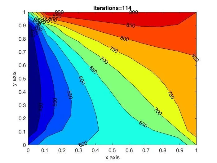
Steady state -
Jacobi -
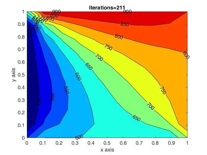
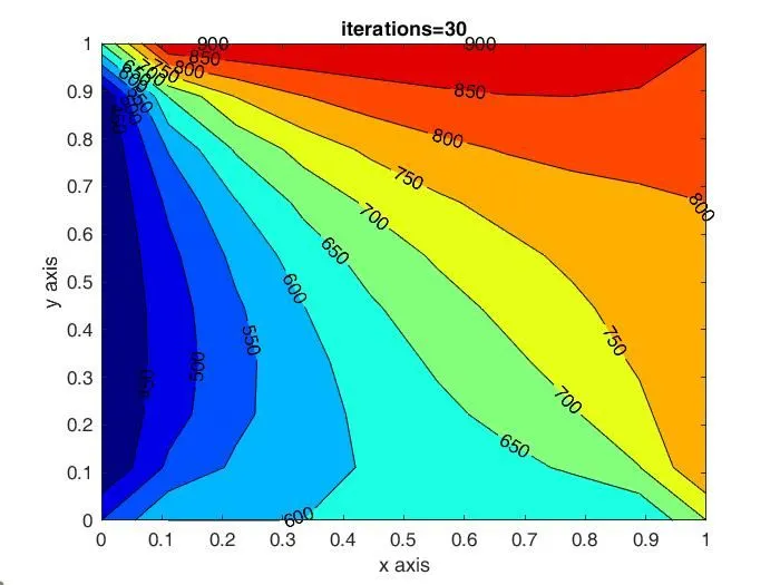
Gauss-Seidel -
SOR -
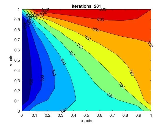
Transient state(Implicit) -
Jacobi -
Gauss-Seidel -
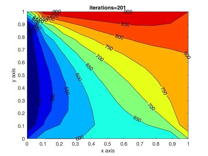
SOR -
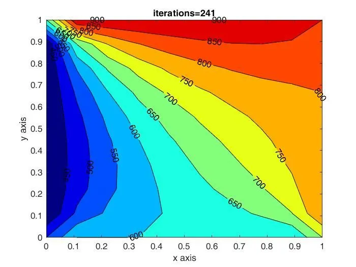
Transient state(Explicit) -
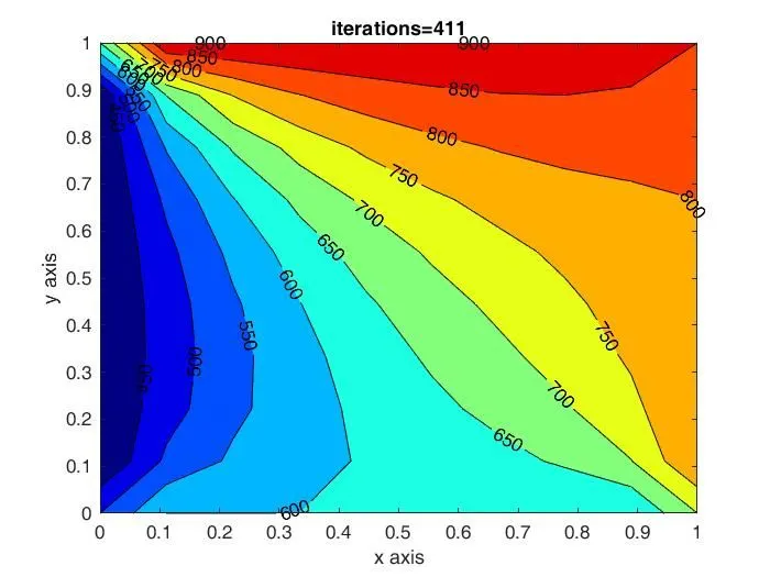
In this study, we studied three different iterative method to find temperature. We can infer from the results the SOR method is best for accuracy and it takes less iteration compare to other two, if relaxation factor is taken within permissible limits. We can conclude that iterative methods works very well and we get solution in no time if we able to guess correct initial values. Iterative methods take less time than direct method also, but be aware about accuracy for coarser mesh.