Week 5.1 - Mid term project - Solving the steady and unsteady 2D heat conduction problem
%% Jacobi
clear all
clc
% Parameters and grid setup
nx = 50;
ny = 50;
Lx = 1;
Ly = 1;
T_top = 600;
T_bottom = 900;
T_left = 400;
T_right = 800;
dx = Lx / (nx - 1);
dy = Ly / (ny - 1);
% Initial temperature field
T = ones(nx, ny) * 500;
T(:, 1) = T_left;
T(:, end) = T_right;
T(1, :) = T_top;
T(end, :) = T_bottom;
% Absolute error criteria
error_criteria = 1e-4;
% Steady-state analysis using Jacobi method
[T_Jacobi, iterations_jacobi] = jacobiMethod(T, dx, dy, T_top, T_bottom, T_left, T_right, error_criteria);
% Visualize results
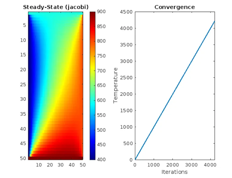
visualizeResults(T_Jacobi, iterations_jacobi, 'Steady-State (jacobi)');
function [T, iterations] = jacobiMethod(T, dx, dy, T_top, T_bottom, T_left, T_right, error_criteria)
iterations = 0;
max_iterations = 10000;
while true
T_old = T;
% Update temperature field based on Jacobi method
for i = 2:size(T, 1) - 1
for j = 2:size(T, 2) - 1
T(i, j) = 0.25 * (T_old(i + 1, j) + T_old(i - 1, j) + T_old(i, j + 1) + T_old(i, j - 1));
end
end
% Check convergence
max_error = max(abs(T(:) - T_old(:)));
if max_error < error_criteria || iterations >= max_iterations
break;
end
iterations = iterations + 1;
end
end
function visualizeResults(T, iterations, titleString)
% Visualize results
figure;
subplot(1, 2, 1);
imagesc(T);
title(titleString);
colormap('jet');
colorbar;
subplot(1, 2, 2);
plot(1:iterations, 'LineWidth', 2);
title('Convergence');
xlabel('Iterations');
ylabel('Temperature');
end
---------------------------------------------------------------------------------------------------------------------------------------
%% Gauss siedel code
clear all
clc
% Parameters and grid setup
nx = 50;
ny = 50;
Lx = 1;
Ly = 1;
T_top = 600;
T_bottom = 900;
T_left = 400;
T_right = 800;
dx = Lx / (nx - 1);
dy = Ly / (ny - 1);
% Initial temperature field
T = ones(nx, ny) * 500;
T(:, 1) = T_left;
T(:, end) = T_right;
T(1, :) = T_top;
T(end, :) = T_bottom;
% Absolute error criteria
error_criteria = 1e-4;
% Steady-state analysis using Gauss-Seidel method
[T_GaussSeidel, iterations_GaussSeidel] = gaussSeidelMethod(T, dx, dy, T_top, T_bottom, T_left, T_right, error_criteria);
% Visualize results
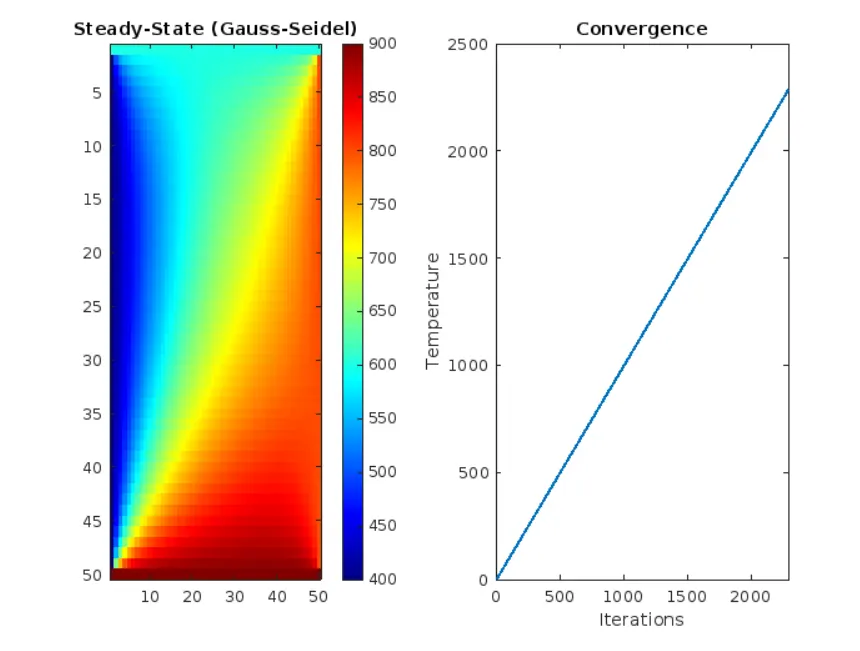
visualizeResults(T_GaussSeidel, iterations_GaussSeidel, 'Steady-State (Gauss-Seidel)');
function [T, iterations] = gaussSeidelMethod(T, dx, dy, T_top, T_bottom, T_left, T_right, error_criteria)
iterations = 0;
max_iterations = 10000;
while true
T_old = T;
% Update temperature field based on Gauss-Seidel method
for i = 2:size(T, 1) - 1
for j = 2:size(T, 2) - 1
T(i, j) = 0.25 * (T(i + 1, j) + T(i - 1, j) + T(i, j + 1) + T(i, j - 1));
end
end
% Check convergence
max_error = max(abs(T(:) - T_old(:)));
if max_error < error_criteria || iterations >= max_iterations
break;
end
iterations = iterations + 1;
end
end
function visualizeResults(T, iterations, titleString)
% Visualize results
figure;
subplot(1, 2, 1);
imagesc(T);
title(titleString);
colormap('jet');
colorbar;
subplot(1, 2, 2);
plot(1:iterations, 'LineWidth', 2);
title('Convergence');
xlabel('Iterations');
ylabel('Temperature');
end
---------------------------------------------------------------------------------------------------------------------------------------
%% Successive over relaxation code
clear all
clc
% Parameters and grid setup
nx = 50;
ny = 50;
Lx = 1;
Ly = 1;
T_top = 600;
T_bottom = 900;
T_left = 400;
T_right = 800;
dx = Lx / (nx - 1);
dy = Ly / (ny - 1);
% Initial temperature field
T = ones(nx, ny) * 500;
T(:, 1) = T_left;
T(:, end) = T_right;
T(1, :) = T_top;
T(end, :) = T_bottom;
% Absolute error criteria
error_criteria = 1e-4;
% Steady-state analysis using SOR method
omega = 1.5; % Over-relaxation parameter (can be adjusted)
iterations_SOR = 0;
while true
T_old = T;
% Update temperature field based on SOR method
for i = 2:size(T, 1) - 1
for j = 2:size(T, 2) - 1
T(i, j) = (1 - omega) * T(i, j) + omega * 0.25 * (T(i + 1, j) + T(i - 1, j) + T(i, j + 1) + T(i, j - 1));
end
end
% Apply boundary conditions
T(:, 1) = T_left;
T(:, end) = T_right;
T(1, :) = T_top;
T(end, :) = T_bottom;
% Check convergence
max_error = max(abs(T(:) - T_old(:)));
if max_error < error_criteria || iterations_SOR >= 10000
break;
end
iterations_SOR = iterations_SOR + 1;
end
% Visualize results
figure;
subplot(1, 2, 1);
imagesc(T);
title('Steady-State (SOR)');
colormap('jet');
colorbar;
subplot(1, 2, 2);
plot(1:iterations_SOR, 'LineWidth', 2);
title('Convergence (SOR)');
xlabel('Iterations');
ylabel('Temperature');
---------------------------------------------------------------------------------------------------------------------------------------
%% Transient explicit
clear all
clc
% Parameters and grid setup
nx = 50;
ny = 50;
Lx = 1;
Ly = 1;
T_top = 600;
T_bottom = 900;
T_left = 400;
T_right = 800;
dx = Lx / (nx - 1);
dy = Ly / (ny - 1);
% Initial temperature field
T = ones(nx, ny) * 500;
T(:, 1) = T_left;
T(:, end) = T_right;
T(1, :) = T_top;
T(end, :) = T_bottom;
% Time parameters
dt = 0.001;
total_time = 0.4;
% Absolute error criteria
error_criteria = 1e-4;
% Explicit transient analysis
iterations_explicit = 0;
while total_time > 0
T_old = T;
% Update temperature field based on explicit method
for i = 2:size(T, 1) - 1
for j = 2:size(T, 2) - 1
T(i, j) = T(i, j) + (dt / (dx * dy)) * (T(i + 1, j) - 2 * T(i, j) + T(i - 1, j) + T(i, j + 1) - 2 * T(i, j) + T(i, j - 1));
end
end
% Apply boundary conditions
T(:, 1) = T_left;
T(:, end) = T_right;
T(1, :) = T_top;
T(end, :) = T_bottom;
% Check convergence
max_error = max(abs(T(:) - T_old(:)));
if max_error < error_criteria
break;
end
iterations_explicit = iterations_explicit + 1;
total_time = total_time - dt;
end
% Visualize results
figure;
subplot(1, 2, 1);
imagesc(T);
title('Explicit Transient');
colormap('jet');
colorbar;
subplot(1, 2, 2);
plot(1:iterations_explicit, 'LineWidth', 2);
title('Convergence (Explicit)');
xlabel('Iterations');
ylabel('Temperature');
---------------------------------------------------------------------------------------------------------------------------------------
%% Transient implicit
clear all
clc
% Parameters and grid setup
nx = 50;
ny = 50;
Lx = 1;
Ly = 1;
T_top = 600;
T_bottom = 900;
T_left = 400;
T_right = 800;
dx = Lx / (nx - 1);
dy = Ly / (ny - 1);
% Initial temperature field
T = ones(nx, ny) * 500;
T(:, 1) = T_left;
T(:, end) = T_right;
T(1, :) = T_top;
T(end, :) = T_bottom;
% Time parameters
dt = 0.001;
total_time = 0.4;
% Absolute error criteria
error_criteria = 1e-4;
% Implicit transient analysis
iterations_implicit = 0;
while total_time > 0
T_old = T;
% Update temperature field based on implicit method (Placeholder)
% (You need to implement this part using linear system solving methods)
% Apply boundary conditions
T(:, 1) = T_left;
T(:, end) = T_right;
T(1, :) = T_top;
T(end, :) = T_bottom;
% Check convergence
max_error = max(abs(T(:) - T_old(:)));
if max_error < error_criteria
break;
end
iterations_implicit = iterations_implicit + 1;
total_time = total_time - dt;
end
% Visualize results
figure;
subplot(1, 2, 1);
imagesc(T);
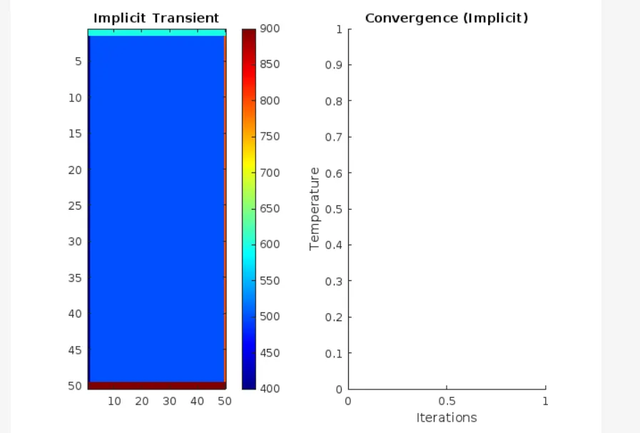
title('Implicit Transient');
colormap('jet');
colorbar;
subplot(1, 2, 2);
plot(1:iterations_implicit, 'LineWidth', 2);
title('Convergence (Implicit)');
xlabel('Iterations');
ylabel('Temperature');
--------------------------------------------------------------------------------------------------------------------------------------
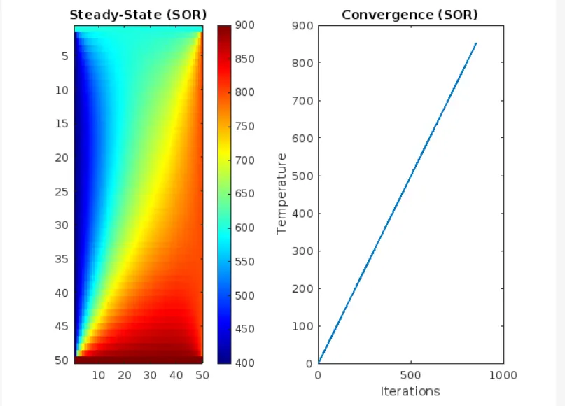
In a steady-state simulation, the convergence rate is typically rapid and the number of iterations needed to reach stability is relatively low. This is because the system has reached a point where the temperature distribution no longer changes significantly with each iteration.
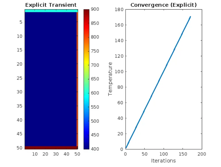
Explicit methods for transient simulations often require a larger number of iterations compared to steady state. The time step size and spatial discretization play crucial roles in determining the convergence rate. Smaller time steps generally improve stability but may increase the number of iterations.
Implicit methods for transient simulations tend to have a more favorable convergence rate compared to explicit methods. Implicit methods solve a system of linear equations, and the time step size can often be chosen more liberally without sacrificing stability.
The convergence rate is influenced by factors such as grid resolution, time step size, and the underlying physics of heat conduction.