Week 5.1 - Mid term project - Solving the steady and unsteady 2D heat conduction problem

2D Heat Conduction equation :

The 2D heat conduction equation describes how temperature changes over time in a two-dimensional space. It is a partial differential equation that governs the distribution of heat within a material. The equation is derived from the principles of conservation of energy and Fourier's law of heat conduction. The general form of the 2D heat conduction equation is:

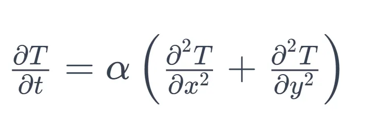
Here, T is the temperature as a function of both spatial coordinates x and y, t is time, and alpha is the thermal diffusivity of the material.

The equation models the evolution of temperature in a two-dimensional space over time. Solving this equation numerically allows one to simulate and analyze the temperature distribution within a physical system, such as a solid object, in response to initial conditions and boundary conditions. It finds applications in various fields, including engineering, physics, and environmental science, where understanding heat transfer is essential. Numerical methods like finite difference, finite element, and finite volume are commonly employed to solve the 2D heat conduction equation in practical scenarios.

Functions code :

Jacobi :

Gauss Seidel :

Succesive Over Relaxation :

Matlab code :

clear all

close all

clc

%inputs

%grid points along x and y axis

nx=10;

ny=10;

x=linspace(0,1,nx);

dx=x(2)-x(1);

y=linspace(0,1,ny);

dy=y(2)-y(1);

%initial temperature values for all nodes

T=300*ones(nx,ny);

%initial boundary condition at the top and botttom

T(1,:)=600;

T(end,:)=900;

%initial boundary condition at the left and right

T(:,1)=400;

T(:,end)=800;

%copy temperature to compute

T_old=T;

T_prev=T;

% initializing error value

error=9e9;

tolerance=1e-4;

omega=1.2;

for iterative_solver=1:3

if iterative_solver==1

iter=1;

while error>tolerance

for i=2:nx-1

for j=2:ny-1

T(i,j)=jacobi(T,T_old,i,j);

end

end

error=max(max(abs(T_old-T)));

%updating value of T

T_old=T;

figure(1)

[u,v]=meshgrid(x,y);

[c,h]= contourf(u,v,T);

colorbar

colormap("jet")

clabel(c,h)

set(gca,'ydir','reverse')

iter_method=sprintf('jacobi iteration is:%d',iter);

title(iter_method);

iter=iter+1;

end

elseif iterative_solver==2

T_old=T_prev;

iter1=1;

while error>tolerance

for i=2:nx-1

for j=2:ny-1

T(i,j)=GS(T,T_old,i,j);

end

end

error=max(max(abs(T_old-T)));

%updating value of T

T_old=T;

figure(2)

[u,v]=meshgrid(x,y);

[c,h]=contourf(u,v,T);

colorbar

colormap("jet")

set(gca,'ydir','reverse')

clabel(c,h)

iter_method=sprintf('GS iteration is:%d',iter1);

title(iter_method);

iter1=iter1+1;

end

elseif iterative_solver==3

iter2=1;

T_old=T_prev;

while error>tolerance

for i=2:nx-1

for j=2:ny-1

T(i,j)=sor(T,T_old,i,j,omega);

end

end

error=max(max(abs(T_old-T)));

%updating value of T

T_old=T;

figure(3)

[u,v]=meshgrid(x,y);

[c,h]= contourf(u,v,T);

colorbar

colormap("jet")

set(gca,'ydir','reverse')

clabel(c,h);

iter_method=sprintf('sor iteration is:%d',iter2);

title(iter_method);

iter2=iter2+1;

end

end

error=9e9;

T_old=T;

end

Gauss Seidel :

Successive over relaxation :

Unsteady Equations

Explicit Method

Matlab code :

close all

clear all

clc

% Transient State Heat Conduction

% dt^2/dT^2 + aplha(d^2T/dx^2 + d^2T/dy^2)=0

nx = 10;

ny = 10;

T = 450*ones(nx,ny);

TL = 400;

TR = 800;

TT = 600;

TB = 900;

% Boundary Conditions

T(:,1) = TL;

T(:,ny) = TR;

T(1,:) = TT;

T(nx,:) = TB;

% Edge Refinement

T(1,1) = (T(1,2)+T(2,1))/2;

T(1,ny) = (T(1,(ny-1))+T(2,ny))/2;

T(nx,1) = (T((nx-1),1)+T(nx,2))/2;

T(nx,ny) = (T(nx,(ny-1))+T((nx-1),ny))/2;

% Inputs

% Time Step

dt = 1e-2;

% Grid Spacing

dx = 1.3e-2;

dy = 1.3e-2;

% Thermal Diffusibility

alpha = 0.004;

k1 = alpha*dt/dx^2;

k2 = alpha*dt/dy^2;

cfl = k1 + k2

% Copy of previous result %

T_previous = T;

conv = 9e9;

tol = 1e-4;

time_iteration = 0;

% Time Looping %

while (conv > tol)

for i = 2:nx-1

for j = 2:ny-1

T(i,j) = (1-2*k1-2*k2)*T_previous(i,j) + k1*(T_previous(i+1,j)+ T_previous(i-1,j)) +k2*(T_previous(i,j+1) + T_previous(i,j-1));

end

end

conv = max(max(abs(T-T_previous)));

T_previous = T;

time_iteration = time_iteration +1;

figure(1)

contourf(flipud(T),'ShowText','ON')

title(sprintf('Transient Explicit Iteration = %d',time_iteration));

pause(0.003)

end

colorbar

Implicit method

Matlab code :

close all

clear all

clc

% Transient State Heat Conduction

% dt^2/dT^2 + aplha(d^2T/dx^2 + d^2T/dy^2) = 0)

nx = 10;

ny = 10;

T = 450*ones(nx,ny);

TL = 400;

TR = 800;

TT = 600;

TB = 900;

% Boundary Conditions

T(:,1) = TL;

T(:,ny) = TR;

T(1,:) = TT;

T(nx,:) = TB;

% Edge Refinement

T(1,1) = (T(1,2)+T(2,1))/2;

T(1,ny) = (T(1,(ny-1))+T(2,ny))/2;

T(nx,1) = (T((nx-1),1)+T(nx,2))/2;

T(nx,ny) = (T(nx,(ny-1))+T((nx-1),ny))/2;

% Inputs from Assesment %

% Time Step for iterations

dt = 1e-2;

% Grid Spacing for accurate results

dx = 1e-2;

dy = 1e-2;

% Thermal Diffusibility constant

alpha = 1.5;

k1 = alpha*dt/dx^2

k2 = alpha*dt/dy^2

% Saving a Copy

Told = T;

T_initial = T;

T_prev = T;

error = 9e9;

conv = 9e9;

tol = 1e-4;

% Iteration Solvers - Jacobi || GS || SOR

% 1- Jacobi Method

jacobi_iteration = 0;

jacobi_time_iterations = 0;

% Time Loop for iterations %

while (conv > tol)

% Space Loop

while (error > tol)

for i = 2:nx-1

for j = 2:ny-1

T(i,j) = (1+2*k1+2*k2)^-1 *(T_prev(i,j)+ k1*(Told(i+1,j)+ Told(i-1,j)) +k2*(Told(i,j+1) + Told(i,j-1)));

end

end

error = max(max(abs(T-Told)));

Told = T;

jacobi_iteration = jacobi_iteration +1;

figure(1)

contourf(flipud(T),'ShowText','ON')

title(sprintf('Transient Implicit Jacobi Iteration = %d \n Time Iteration = %d',jacobi_iteration,jacobi_time_iterations));

pause(0.003)

end

conv = max(max(abs(T-T_prev)));

T_prev = T;

jacobi_time_iterations = jacobi_time_iterations +1;

error = 9e9;

end

colorbar

% Reinitialising the old values %

T = T_initial;

Told = T;

T_prev = T;

error = 9e9;

conv = 9e9;

% 2 ------ Gauss Seidel Method %

gs_iteration = 0;

gs_time_iteration =0;

% Time Loop

while (conv > tol)

% Space Loop

while (error > tol)

for i = 2:nx-1

for j = 2:ny-1

T(i,j) = (1+2*k1+2*k2)^-1 *(T_prev(i,j)+ k1*(Told(i+1,j)+ T(i-1,j)) +k2*(Told(i,j+1) + T(i,j-1)));

end

end

error = max(max(abs(T-Told)));

Told = T;

gs_iteration = gs_iteration +1;

figure(2)

contourf(flipud(T),'ShowText','ON')

title(sprintf('Transient Implicit Gauss Seidel Iteration = %d \n Time Iteration = %d',gs_iteration,gs_time_iteration));

pause(0.003)

end

conv = max(max(abs(T-T_prev)));

T_prev = T;

gs_time_iteration = gs_time_iteration +1;

error = 9e9;

end

colorbar

% Reinitialising

T = T_initial;

Told = T;

T_prev = T;

error = 9e9;

conv = 9e9;

% 3- Successive over-relaxation (SOR)

sor_iteration = 0;

sor_time_iteration = 0;

omega = 1.5;

% Time Loop

while (conv > tol)

% Space Loop

while (error > tol)

for i = 2:nx-1

for j = 2:ny-1

TGS(i,j) = (1+2*k1+2*k2)^-1 *(T_prev(i,j)+ k1*(Told(i+1,j)+ T(i-1,j)) +k2*(Told(i,j+1) + T(i,j-1)));

T(i,j) = (1-omega)*Told(i,j) + omega*TGS(i,j);

end

end

error = max(max(abs(T-Told)));

Told = T;

sor_iteration = sor_iteration +1;

figure(3)

contourf(flipud(T),'ShowText','ON')

title(sprintf('Transient Implicit Successive over-relaxation Iteration = %d \n Time Iteration = %d',sor_iteration,sor_time_iteration));

pause(0.003)

end

conv = max(max(abs(T-T_prev)));

T_prev = T;

sor_time_iteration = sor_time_iteration +1;

error = 9e9;

end

colorbar

Jacobi :

Gauss seidel :

Succesive over relaxation :

Results:

1. Steady-State Simulations:

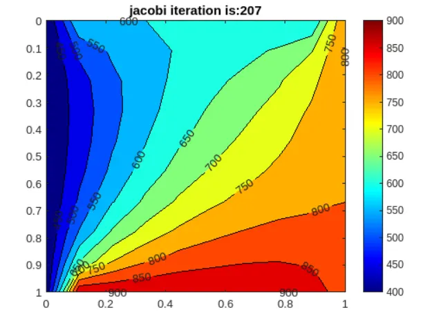
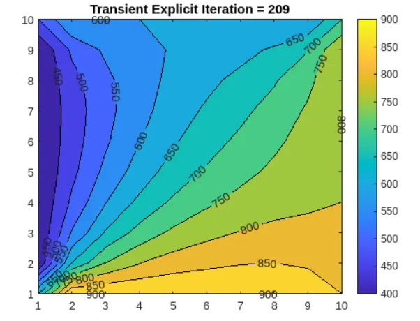
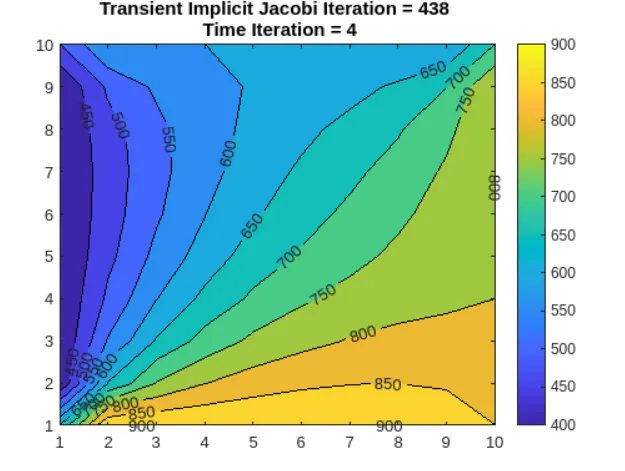
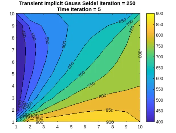
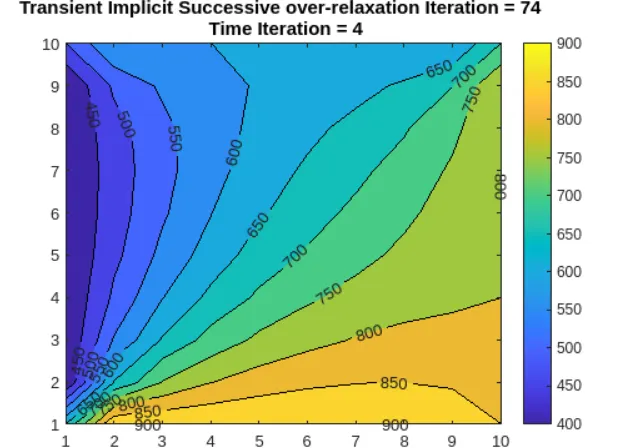
• Jacobi Method: It is the slowest among the three methods, as it updates the entire grid at each iteration. Convergence is achieved through a large number of iterations, and each iteration involves updating the entire grid.
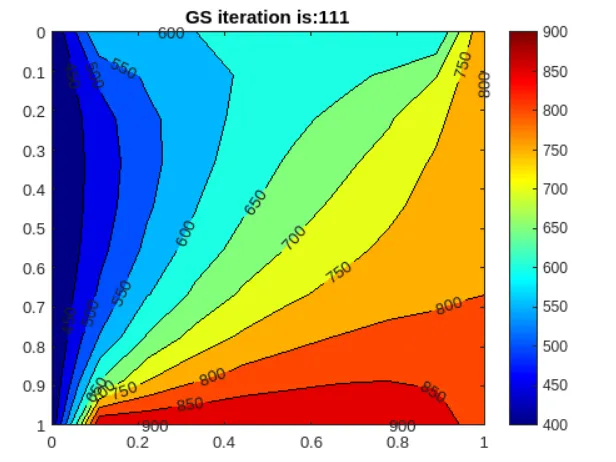
• Gauss-Seidel Method: It is faster than Jacobi, as it updates the grid in a more sequential manner. The new values are used immediately, leading to a quicker convergence compared to Jacobi.
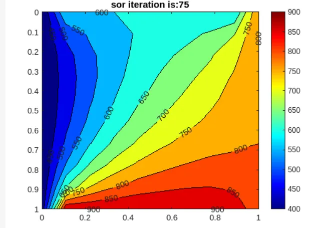
• Successive Over Relaxation (SOR): SOR introduces a relaxation factor (omega) to speed up convergence. It is expected to converge faster than Gauss-Seidel and Jacobi. The choice of omega affects the convergence rate.

2. Transient Simulations:

• Explicit Method: This method involves updating the temperature at each grid point explicitly based on the previous time step. The stability of the solution depends on the Courant-Friedrichs-Lewy (CFL) condition. It is conditionally stable, and a small time step is required for stability. The convergence is achieved through time iterations.
• Implicit Method (Jacobi, Gauss-Seidel, SOR): Implicit methods involve solving a system of linear equations at each time step. They offer unconditional stability and larger time steps compared to explicit methods. However, each time step involves solving a system, making it computationally more expensive.

Conclusion:

• For steady-state simulations, SOR is expected to converge faster than Gauss-Seidel, and Gauss-Seidel is expected to converge faster than Jacobi. The choice of method depends on the problem size and desired accuracy.
• For transient simulations, the implicit methods (Jacobi, Gauss-Seidel, SOR) are more stable and allow for larger time steps compared to the explicit method. Among the implicit methods, SOR may converge faster due to the relaxation factor.
• The convergence rates are influenced by factors such as grid resolution, boundary conditions, and the choice of relaxation parameters (omega for SOR).
• Adjustments to the numerical parameters(e.g.,time step,grid spacing) and the choice of iterative solvers can significantly impact the convergence behaviour.