Week 5.1 - Mid term project - Solving the steady and unsteady 2D heat conduction problem

Mid-term project - Solving the steady and unsteady 2D heat conduction problem

Aim:

1. Solve the 2D heat conduction equation by using the point iterative techniques that were taught in class. The Boundary conditions for the problem are as follows;

Top Boundary = 600 K

Bottom Boundary = 900 K

Left Boundary = 400 K

Right Boundary = 800 K

By implementing the following methods for solving implicit equations.

• Jacobi
• Gauss-seidel
• Successive over-relaxation

2. Write code for both implicit and explicit schemes (This is for the transient analysis only)

3. Compare the convergence rate [Number of iterations] of the steady state and transient [explicit and implicit] simulations and justify the numerics.

HINT:

Introduction:

Implicit Iterative Solver

When solving partial differential equations (PDEs) numerically, an implicit method takes into account the links between several places in a discretized domain.

In contrast to other methods, the implicit approach has the advantage of computing the new values of the solution variables based on relationships involving neighboring places. Whereas explicit methods where the new values are only dependent on the current values of surrounding places, implicit procedures need the solution of a set of equations to arrive at the new values.

In this code, an implicit solver is employed to simulate heat conduction and solve the steady-state temperature distribution.

Domain Discretization: A grid of dots along the x and y axes represents the domain. In order to do this, arrays x and y that reflect the grid points' spatial coordinates must be created.
Boundary Conditions: The initial temperature matrix t is populated with default values (300K) and boundary conditions are set. These conditions determine the temperature at the edges of the domain.

Iteration and Implicit Update: The main iteration loop updates the temperature values using an implicit approach. This involves setting up and solving a system of equations based on the discretized heat conduction equation.

Convergence Criteria: The iteration continues until a convergence criterion is met. The maximum difference between the current and previous temperature values (error) is compared to a specified tolerance. When the error falls below the tolerance, the iteration stops.

After convergence, a contour map is used to display the resultant temperature distribution. Labels, a colour bar, and other pertinent information are included in the code that creates a contour map of temperature readings.

Jacobi iterative solver Method:

A numerical method for solving linear systems of equations iteratively is the Jacobi iterative solver. In numerical simulations of partial differential equations, such as heat conduction, it is frequently used. The approach uses the average of nearby values from the prior iteration to update each unknown variable throughout each iteration. Although Jacobi offers simplicity and computation independence, its convergence may be slower than those of other approaches. Nevertheless, it continues to be significant due to its simple implementation and parallelizability, making it a key tool in simulations and scientific computing.

Gauss-Seidel iterative solver Method:

A refined Jacobi approach, Gauss-Seidel updates variables using the latest values, enhancing convergence by exploiting current information. Effective for diagonally dominant systems, it's widely used for solving linear and nonlinear equations, though it sacrifices some parallelism for faster convergence.

Successive Over-Relaxation (SOR) iterative solver Method:

The Gauss-Seidel technique is extended with a relaxation factor by the Successive Over-Relaxation (SOR) iterative solver. By modifying the updates according to a user-defined factor, it hastens convergence. SOR integrates data from past and present iterations, increasing convergence for well-behaved systems and aiding in the resolution of slow convergence problems in conventional Gauss-Seidel.

The method is particularly effective when used on problems with irregularities or when fine-tuning convergence speed is necessary. SOR's balance between stability and convergence speed makes it a valuable tool in various scientific and engineering simulations, aiding in solving linear systems and PDEs.

Steady State

`∂^2T∂x^2+∂^2T∂y^2=0`

`∂^2T∂x^2=underset(i−1,j)T+2underset(i,j)T+underset(i+1,j)T.δx^2`

`∂^2T∂y^2=underset(i,j−1)T+2underset(i,j)T+underset(i,j+1)T.δy^2`

Jacobi iterative solver Method

`underset(i,j)T=`underset(i−1,j)T+underset(i+1,j)T.k⋅dx^2+underset(i,j−1)T+underset(i,j−1,old)T.k⋅dy2^)`

`Where k=(2(∂x^2+∂y^2))/(∂x^2⋅∂y^2)`

2. Gauss-Seidel iterative solver Method:

`underset(i,j)T=(underset(i−1,j,old)T+underset(i+1,j)Tk⋅dx^2+underset(i,j−1,old)T+underset(i,j−1)T.k⋅dy^2)`

`Where k=(2(∂x^2+∂y^2))/(∂x^2⋅∂y^2)`

3. Successive Over-Relaxation (SOR) iterative solver Method:

`underset(i,j)T=(1−ω)underset(i,j,old)T+ω(underset(i−1,j,old)T+underset(i+1,j)T.k⋅dx^2+underset(i,j−1,old)T+underset(i,j−1)T.k⋅dy^2)`

`Where k=(2(∂x^2+∂y^2))/(∂x^2⋅∂y^2)`

Matlab Code

% Clear previous data, figures, and console
clear all
close all
clc

% Steady state analysis

nx = 100; % number of grid points
x = linspace(0, 1, nx); % Generating spatial coordinates along x
dx = x(2) - x(1); % Grid spacing
dy = dx; % Assumption: Equal spacing in x and y
y = linspace(0, 1, nx); % Generating spatial coordinates along y

T = 300 * ones(nx, nx); % Initial temperature condition (in Kelvin)
T(:, 1) = 400; % Left boundary temperature (K)
T(end, :) = 600; % Top boundary temperature (K)
T(:, end) = 800; % Right boundary temperature (K)
T(1, :) = 900; % Bottom boundary temperature (K)

tol = 1e-4; % Absolute error criteria for convergence
Told1 = T; Told2 = T; Told3 = T; % Store previous temperature matrices
T1 = T; T2 = T; T3 = T; % Current temperature matrices for each method

% Loop over methods: 1.Jacobi, 2.Gauss-Seidel, 3.Successive Over Relaxation (SOR)
for method = 1:25

    % Jacobi method
    if method == 1
        jac_error = 1e9; % Initialize error
        jacobi_iter = 0; % Initialize iteration count
        tic % Start timing
        while jac_error > tol 
            jacobi_iter = jacobi_iter + 1;
            for i = 2:(nx-1)
                for j = 2:(nx-1)
                    % Update temperature using Jacobi method
                    T1(i, j) = (Told1(i-1, j) + Told1(i+1, j) + Told1(i, j-1) + Told1(i, j+1)) / 4;
                end
            end
            jac_error = max(max(abs(T1 - Told1)));
            Told1 = T1;
        end
        analysis_time1 = toc; % Stop timing
        % Visualize temperature distribution and details
        figure(1);
        contourf(x, y, T1, 'Showtext', 'on');
        colormap(hsv);
        c=colorbar;
        c.Label.String= 'Temperature in Kelvin(K)';
        xlabel('X axis');
        ylabel('Y axis');
        title(sprintf('2D Steady State Analysis (Jacobi Method) \nTemperature Distribution over a Plate \nIterations: %dnAnalysis Time: %.4f seconds', jacobi_iter, analysis_time1));
        pause(0.1);
        
    % Gauss-Seidel method
    elseif method == 2
        % Similar loop structure as Jacobi, with updated values used immediately
        gauss_error = 1e9; % Initialize error
        gauss_iter = 0; % Initialize iteration count
        tic % Start timing
        while gauss_error > tol 
            gauss_iter = gauss_iter + 1;
            for i = 2:(nx-1)
                for j = 2:(nx-1)
                    % Update temperature using Gauss-Seidel method
                    T2(i, j) = (T2(i-1, j) + Told2(i+1, j) + T2(i, j-1) + Told2(i, j+1)) / 4;
                end
            end
            gauss_error = max(max(abs(T2 - Told2)));
            Told2 = T2;
        end
        analysis_time2 = toc; % Stop timing
        % Visualize temperature distribution and details
        figure(2);
        contourf(x, y, T2, 'Showtext', 'on');
        colormap(hsv);
        c=colorbar;
        c.Label.String= 'Temperature in Kelvin(K)';
        xlabel('X axis');
        ylabel('Y axis');
        title(sprintf('2D Steady State Analysis (Gauss Seidel Method) \nTemperature Distribution over a Plate \nIterations: %dnAnalysis Time: %.4f seconds', gauss_iter, analysis_time2));
        pause(0.1);
        
    % Successive Over-Relaxation (SOR) method
    elseif method == 3
        w = 2 / (1 + sin(pi * dx)); % Relaxation parameter
        sor_error = 1e9; % Initialize error
        sor_iter = 0; % Initialize iteration count
        tic % Start timing
        while sor_error > tol 
            sor_iter = sor_iter + 1;
            for i = 2:(nx-1)
                for j = 2:(nx-1)
                    % Update temperature using SOR method
                    T3(i, j) = (1 - w) * T3(i, j) + w * (T3(i-1, j) + Told3(i+1, j) + T3(i, j-1) + Told3(i, j+1)) / 4;
                end
            end
            sor_error = max(max(abs(Told3 - T3)));
            Told3 = T3;
        end
        analysis_time3 = toc; % Stop timing
        % Visualize temperature distribution and details
        figure(3);
        contourf(x, y, T3, 'Showtext', 'on');
        colormap(hsv);
        c=colorbar;
        c.Label.String= 'Temperature in Kelvin(K)';
        xlabel('X axis');
        ylabel('Y axis');
        title(sprintf('2D Steady State Analysis (SOR Method)\nTemperature Distribution over a Plate \nIterations: %dnAnalysis Time: %.4f seconds', sor_iter, analysis_time3));
        pause(0.1);
    end
end

Output:

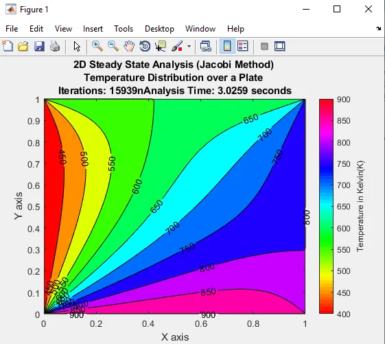
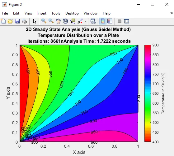
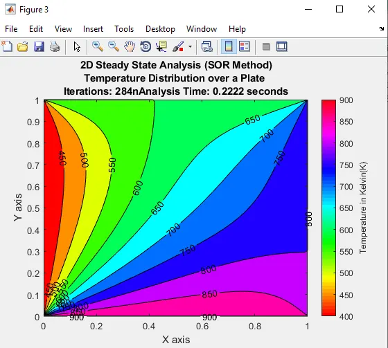
TRANSIENT STATE ANALYSIS:

Explicit Method Matlab Code:

clear all
close all
clc

% transient heat conduction

nx = 100; % number of grid points
x = linspace(0,1,nx);   % Spatial coordinates along x-axis
dx = x(2) - x(1);       % Grid spacing
dy = dx;                % Equal spacing assumption in x and y
y = linspace(0,1,nx);   % Spatial coordinates along y-axis
total_time = 10;        % Total simulation time
dt = 0.01;              % Time step
total_time_steps = total_time/dt;% Total time steps

T = 300*ones(nx,nx); % initial temperature condition
T(:,1) = 400; % K ,temperature left boundary condition
T(end,:) = 600; % K ,temperature top boundary condition
T(:,end) = 800; % K ,temperature right boundary condition
T(1,:) = 900; % K ,temperature bottom boundary condition

tol = 1e-5;             % Tolerance for convergence
Alpha = 0.002;          % thermal diffusivity
k = Alpha*dt/(dx^2);    % Diffusion coefficient
CFL = Alpha*dt/(dx^2);  % CFL number

% Initialize matrices to store previous and current temperature values
Told1 = T; Told2 = T; Told3 = T; Told4 = T;
T1 = T; T2 = T; T3 = T; T4 = T;
T_time1  = T; T_time2 = T; T_time3 = T; T_time4 = T; % for time loop

for method = 1:4
    
    % 1.transient explicit
 
  if method ==1
       cycle = 0;                   % Initialize cycle count
        tic                         % Start timing
        for t = 1:total_time_steps
            for i = 2:(nx-1)
                for j = 2:(nx-1)
                    % Update temperature using explicit method
                    T1(i,j) = Told1(i,j) + k*(Told1(i-1,j) + Told1(i+1,j) + Told1(i,j-1) + Told1(i,j+1)-4*Told1(i,j));
                end
            end
            Told1 = T1; 
            cycle = cycle + 1;
        end
        convergence_time1 = toc;    % Stop timing
        figure(1)
        contourf(x,y,T1,'Showtext','on')
        colormap(hsv)
        c=colorbar;
        c.Label.String= 'Temperature in Kelvin(K)';
        xlabel('X axis')
        ylabel('Y axis')
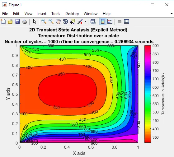
        title(sprintf('2D Transient State Analysis (Explicit Method) \nTemperature Distribution over a plate \nNumber of cycles = %d nTime for convergence = %f seconds',cycle,convergence_time1))
        pause(0.2)
  end
end

Output

Implicit Method Matlab Code:

Jacobi iterative solver Method

clear all
close all
clc

% transient heat conduction

nx = 100; % number of grid points
x = linspace(0,1,nx);   % Spatial coordinates along x-axis
dx = x(2) - x(1);       % Grid spacing
dy = dx;                % Equal spacing assumption in x and y
y = linspace(0,1,nx);   % Spatial coordinates along y-axis
total_time = 10;        % Total simulation time
dt = 0.01;              % Time step
total_time_steps = total_time/dt;% Total time steps

T = 300*ones(nx,nx); % initial temperature condition
T(:,1) = 400; % K ,temperature left boundary condition
T(end,:) = 600; % K ,temperature top boundary condition
T(:,end) = 800; % K ,temperature right boundary condition
T(1,:) = 900; % K ,temperature bottom boundary condition

tol = 1e-5;             % Tolerance for convergence
Alpha = 0.002;          % thermal diffusivity
k = Alpha*dt/(dx^2);    % Diffusion coefficient
CFL = Alpha*dt/(dx^2);  % CFL number

% Initialize matrices to store previous and current temperature values
Told1 = T; Told2 = T; Told3 = T; Told4 = T;
T1 = T; T2 = T; T3 = T; T4 = T;
T_time1  = T; T_time2 = T; T_time3 = T; T_time4 = T; % for time loop

% transient implicit jacobi
       tic
       for t = 1:total_time_steps
           jacobi_error = 1e9;
           jacobi_iter = 0;
           while (jacobi_error>tol)
               jacobi_iter = jacobi_iter + 1;
               for i = 2:(nx-1)
                   for j = 2:(nx-1)
                       T2(i,j) = T_time2(i,j)/(1+4*k) + (k/(1+4*k))*(Told2(i-1,j) + Told2(i+1,j) + Told2(i,j-1) + Told2(i,j+1));
                   end
               end
               jacobi_error = max(max(abs(T2-Told2)));
               Told2 = T2;
           end
           T_time2 = T2;
       end
        convergence_time2 = toc;
        figure(2)
        contourf(x,y,T2,'Showtext','on')
        colormap(hsv)
        c=colorbar;
        c.Label.String= 'Temperature in Kelvin(K)';
        xlabel('X axis')
        ylabel('Y axis')
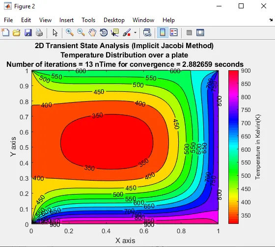
        title(sprintf('2D Transient State Analysis (Implicit Jacobi Method) \nTemperature Distribution over a plate \nNumber of iterations = %d nTime for convergence = %f seconds',jacobi_iter,convergence_time2))
        pause(0.2)

Output

Gauss-Seidel iterative solver Method Matlab Code:

clear all
close all
clc

% transient heat conduction

nx = 100; % number of grid points
x = linspace(0,1,nx);   % Spatial coordinates along x-axis
dx = x(2) - x(1);       % Grid spacing
dy = dx;                % Equal spacing assumption in x and y
y = linspace(0,1,nx);   % Spatial coordinates along y-axis
total_time = 10;        % Total simulation time
dt = 0.01;              % Time step
total_time_steps = total_time/dt;% Total time steps

T = 300*ones(nx,nx); % initial temperature condition
T(:,1) = 400; % K ,temperature left boundary condition
T(end,:) = 600; % K ,temperature top boundary condition
T(:,end) = 800; % K ,temperature right boundary condition
T(1,:) = 900; % K ,temperature bottom boundary condition

tol = 1e-5;             % Tolerance for convergence
Alpha = 0.002;          % thermal diffusivity
k = Alpha*dt/(dx^2);    % Diffusion coefficient
CFL = Alpha*dt/(dx^2);  % CFL number

% Initialize matrices to store previous and current temperature values
Told1 = T; Told2 = T; Told3 = T; Told4 = T;
T1 = T; T3 = T; T3 = T; T4 = T;
T_time1  = T; T_time2 = T; T_time3 = T; T_time4 = T; % for time loop

% transient implicit gauss seidel
       tic
       for t = 1:total_time_steps
           Gauss_seidel_error = 1e9;
           Gauss_seidel_iter = 0;
           while(Gauss_seidel_error>tol)
               Gauss_seidel_iter = Gauss_seidel_iter + 1;
               for i = 2:(nx-1)
                   for j = 2:(nx-1)
                       T3(i,j) = T_time3(i,j)/(1+4*k) + (k/(1+4*k))*(T3(i-1,j) + Told3(i+1,j) + T3(i,j-1) + Told3(i,j+1));
                   end
               end
               Gauss_seidel_error = max(max(abs(Told3-T3)));
               Told3 = T3;
           end
           T_time3 = T3;
       end
        convergence_time3 = toc;
        figure(3)
        contourf(x,y,T3,'Showtext','on')
        colormap(hsv)
        c=colorbar;
        c.Label.String= 'Temperature in Kelvin(K)';
        xlabel('X axis')
        ylabel('Y axis')
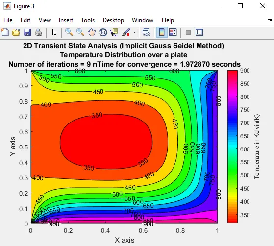
        title(sprintf('2D Transient State Analysis (Implicit Gauss Seidel Method) \nTemperature Distribution over a plate \nNumber of iterations = %d nTime for convergence = %f seconds',Gauss_seidel_iter,convergence_time3))
        pause(0.2)

Output

Successive Over-Relaxation (SOR) iterative solver Method Matlab Code:

clear all
close all
clc

% transient heat conduction

nx = 100; % number of grid points
x = linspace(0,1,nx);   % Spatial coordinates along x-axis
dx = x(2) - x(1);       % Grid spacing
dy = dx;                % Equal spacing assumption in x and y
y = linspace(0,1,nx);   % Spatial coordinates along y-axis
total_time = 10;        % Total simulation time
dt = 0.01;              % Time step
total_time_steps = total_time/dt;% Total time steps

T = 300*ones(nx,nx); % initial temperature condition
T(:,1) = 400; % K ,temperature left boundary condition
T(end,:) = 600; % K ,temperature top boundary condition
T(:,end) = 800; % K ,temperature right boundary condition
T(1,:) = 900; % K ,temperature bottom boundary condition

tol = 1e-5;             % Tolerance for convergence
Alpha = 0.002;          % thermal diffusivity
k = Alpha*dt/(dx^2);    % Diffusion coefficient
CFL = Alpha*dt/(dx^2);  % CFL number

% Initialize matrices to store previous and current temperature values
Told1 = T; Told2 = T; Told3 = T; Told4 = T;
T1 = T; T3 = T; T3 = T; T4 = T;
T_time1  = T; T_time2 = T; T_time3 = T; T_time4 = T; % for time loop

% transient implicit SOR
      w = 2/(1+sin(pi*dx)); % relaxation parameter
      tic
      for t = 1:total_time_steps
          SOR_error = 1e9;
          SOR_iter = 0;
          while (SOR_error>tol)
              SOR_iter = SOR_iter + 1;
              for i = 2:(nx-1)
                  for j = 2:(nx-1)
                      T4(i,j) =(1-w)*Told4(i,j) + w*(T_time4(i,j))/(1+4*k) + w*(k/(1+4*k))*(T4(i-1,j) + Told4(i+1,j) + T4(i,j-1) + Told4(i,j+1));
                  end
              end
              SOR_error = max(max(abs(Told4-T4)));
              Told4 = T4;
          end
          T_time4 = T4;
      end
        convergence_time4 = toc;
        figure(4)
        contourf(x,y,T4,'Showtext','on')
        colormap(hsv)
        c=colorbar;
        c.Label.String= 'Temperature in Kelvin(K)';
        xlabel('X axis')
        ylabel('Y axis')
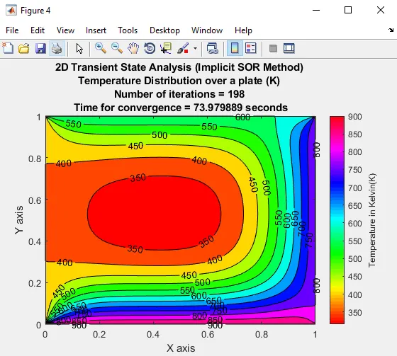
        title(sprintf('2D Transient State Analysis (Implicit SOR Method) \nTemperature Distribution over a plate \nNumber of iterations = %d nTime for convergence = %f seconds',SOR_iter,convergence_time4))
        pause(0.2)

Output

Conclusion

• Firstly, explicit methods exhibit faster convergence compared to implicit ones. Among the implicit techniques, Gauss-Seidel proves to be the instantaneous
  in reaching convergence, followed by the Jacobi method, which outperforms SOR in terms of convergence time.
• In contrast to Gauss-Seidel and SOR, Jacobi's convergence calls for a large number of iterations in the steady-state situation. These iterations can be greatly reduced while maintaining convergence stability by increasing the grid size.
• Explicit and implicit approaches are combined to solve unstable situations in transient state analysis. The explicit technique requires fewer time steps but takes longer to compute for stiff equations. When compared to implicit solutions, SOR provides quick and consistent results while accommodating different CFL values.
• Surprisingly, compared to their steady-state equivalents, implicit approaches for transient state analysis need fewer Jacobi, Gauss-Seidel, and SOR iterations. However, when thermal diffusivity (Alpha) and temporal derivatives are taken into account, convergence time increases.