Week 5.1 - Mid term project - Solving the steady and unsteady 2D heat conduction problem

Theory - Steady State Analysis and Transient State Analysis are two important concepts in engineering and physics, particularly when studying dynamic systems. These terms are often used in various fields, including heat conduction analysis. Let's explore each concept and its application to the 2D heat conduction equation:

1. Steady State Analysis: Steady state analysis refers to the study of a system when it has reached a stable equilibrium, and all variables within the system remain constant with respect to time. In other words, the system's behaviour does not change over time, and there are no transient effects. For instance, if you leave a metal rod in a constant temperature environment for a long time, eventually the temperature distribution along the rod will stabilize, and the heat flow will be constant at any point along its length.
2. Transient State Analysis: Transient state analysis, on the other hand, involves studying a system's behaviour during the time it takes to reach a steady state after some change or disturbance occurs. During the transient state, the system's variables are changing over time until it finally stabilizes. Continuing with the metal rod example, when you suddenly heat one end of the rod, the temperature distribution will change over time until it reaches a steady state with a new temperature profile.

2D Heat Conduction Equation: The 2D heat conduction equation describes the heat transfer in two dimensions (e.g., along the x and y axes) and is commonly represented as:

∂T/∂t = α (∂²T/∂x² + ∂²T/∂y²)

where: T is the temperature distribution function with respect to both x and y coordinates. t is time. α is the thermal diffusivity of the material.

Application to Steady State Analysis: For steady state analysis, we set the left-hand side of the heat conduction equation to zero (∂T/∂t = 0) since there are no time-dependent changes in the temperature. This simplifies the equation to:

0 = α (∂²T/∂x² + ∂²T/∂y²)

The above equation is known as Laplace's equation, which governs the temperature distribution in the steady state.

Application to Transient State Analysis: For transient state analysis, we keep the time-dependent term (∂T/∂t) in the heat conduction equation, as transient effects are considered. Solving the 2D heat conduction equation with initial and boundary conditions yields the transient temperature distribution over time until it reaches a steady state.

Solution- These three methods, Jacobi, Gauss-Seidel, and Successive Over-Relaxation, are iterative techniques used to solve implicit equations, especially when dealing with systems of linear equations. Implicit equations are equations where the variables are not explicitly isolated on one side of the equation. These iterative methods are commonly used in numerical analysis and computational mathematics. Let's explore each method:

1. Jacobi Method: The Jacobi method is an iterative technique used to solve systems of linear equations of the form AX = B, where A is a square matrix, X is the vector of unknowns, and B is the right-hand side vector. In the Jacobi method, the system is transformed into an iteration formula:

X(k+1)_i = (1/A_ii) * (B_i - Σ(A_ij * X(k)_j)), for i = 1, 2, ..., n

where X(k)_i is the i-th component of the vector X at the k-th iteration, A_ii is the diagonal element of matrix A, and A_ij represents the other elements of matrix A. The Jacobi method updates each component of the solution vector simultaneously using the previous iteration's values.

1. Gauss-Seidel Method: Similar to the Jacobi method, the Gauss-Seidel method is another iterative technique used to solve systems of linear equations. It's an improvement over the Jacobi method as it updates the components of the solution vector in-place as soon as new values become available. The iteration formula for the Gauss-Seidel method is:

X(k+1)_i = (1/A_ii) * (B_i - Σ(A_ij * X(k+1)_j) - Σ(A_ij * X(k)_j)), for i = 1, 2, ..., n

In the Gauss-Seidel method, the updated value of each component of the solution vector (X(k+1)_i) is used immediately in the same iteration for calculating the updated values of other components.

1. Successive Over-Relaxation (SOR) Method: The Successive Over-Relaxation method is an extension of the Gauss-Seidel method that introduces an additional relaxation factor (ω) to accelerate convergence. The iteration formula for the SOR method is:

X(k+1)_i = (1 - ω) * X(k)_i + (ω/A_ii) * (B_i - Σ(A_ij * X(k+1)_j) - Σ(A_ij * X(k)_j)), for i = 1, 2, ..., n

The relaxation factor ω allows the method to "overshoot" the update, which can improve the convergence rate for some systems. The optimal value of ω depends on the specific problem and must be chosen carefully to ensure convergence.

% Solving Steady and unsteady 2D heat conduction problem
% Steady state conduction 
% Iterative solver - Jacobi, Gauss -seidel, Relaxation methods

clear all
close all
clc

%initial conditions
%L = 1
nx = 10;
ny = 10;
x = linspace(0,1,nx);
y = linspace(0,1,ny);
dx = x(2) - x(1);
dy = y(2) - y(1);


% given data of boundary condition
% initial temp condition

t = 300*ones(nx,ny);  
t(:,1) = 400;
t(1,:) = 600;
t(:,ny) = 800;
t(nx,:) = 900;

% defining the temperature at corner points

t(1,1) = 500;
t(nx,ny) = 850;
t(1,ny) = 700;
t(nx,1) = 650;

dt = 1e-2; %time step
told=t;

error = 100;
tol = 1e-4;
k = 2*(dx^2+dy^2)/(dx^2*dy^2);
% k2 = (dy^2)/(2*(dx^2+dy^2));

method = input('Iterative method = '); %iterative method selection

%JACOBI ITERATIVE METHOD

if (method==1)
    tic;
    jacobi = 1;
    while(error>tol)
        for i = 2:(nx-1)
            for j = 2:(ny-1)
            t(i,j) = (((told(i-1,j)+told(i+1,j))/(dx^2))+((told(i,j+1)+told(i,j-1))/(dy^2)))/k;
            end
        end
    error = max(max(abs(t-told)));
    told = t;
    jacobi = jacobi+1;
    time_taken = toc;
    end

%plotting    
figure(1)
contourf(x,y,t,'ShowText','on');
colormap(jet);
colorbar;
xlabel('X')
ylabel('Y')
text1 = sprintf('number of iteration = %d', jacobi);
text2 = sprintf('simulation time = %f', time_taken);
title({'Steady state heat condustion profile by jacobi'; text1; text2});
end


%GAUSS-SEIDEL ITERATIVE METHOD

if (method==2)
    tic;
    gauss = 1;
    while(error>tol)
        for i = 2:(nx-1)
            for j = 2:(ny-1)
            t(i,j) = (((t(i-1,j)+told(i+1,j))/(dx^2))+((told(i,j+1)+t(i,j-1))/(dy^2)))/k;
            end
        end
    error = max(max(abs(t-told)));
    told = t;
    gauss = gauss+1;
    time_taken = toc;
    end

%plotting
figure(2)
contourf(x,y,t,'ShowText','on');
colormap(jet);
colorbar;
xlabel('X')
ylabel('Y')
text1 = sprintf('number of iteration = %d', gauss);
text2 = sprintf('simulation time = %f', time_taken);
title({'Steady state heat condustion profile by Gauss-Seidel'; text1; text2});
end


%SUCCESSIVE OVER RELAXATION ITERATIVE METHOD

if (method==3)
    tic;
    sor = 1;
    omega = 1.4; %over relaxation factor
    while(error>tol)
        for i = 2:(nx-1)
            for j = 2:(ny-1)
            term1 =(t(i-1,j)+told(i+1,j))/(dx^2);
            term2 =(told(i,j+1)+t(i,j-1))/(dy^2);
            t(i,j) = ((told(i,j)*(1-omega)))+(omega*(term1+term2))/k;
            end
        end
    error = max(max(abs(t-told)));
    told = t;
    sor = sor+1;
    time_taken = toc;
    end

%plotting
figure(3)
contourf(x,y,t,'ShowText','on');
colormap(jet);
colorbar;
xlabel('X')
ylabel('Y')
text1 = sprintf('number of iteration = %d', sor);
text2 = sprintf('simulation time = %f', time_taken);
text3 = sprintf('over relaxation factor = %f', omega);
title({'Steady state heat condustion profile by Successive Over Relaxation'; text1; text2; text3});
end

Output - 

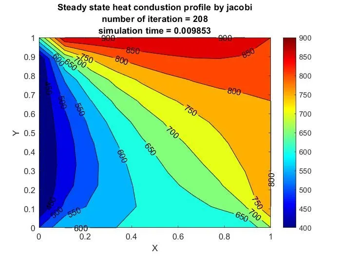
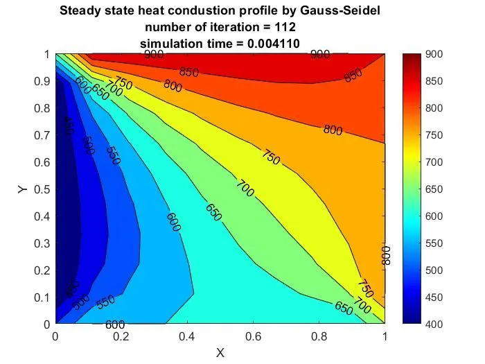
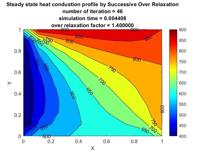
Transient (Unsteady) state simulation:

Explicit and implicit methods are two different approaches used in numerical methods to solve differential equations or systems of equations. These methods are commonly employed in various fields, including physics, engineering, and computational mathematics. Let's understand the key differences between explicit and implicit methods:

1. Explicit Methods: Explicit methods are numerical techniques that calculate the values of the unknowns at the next time step directly from the known values at the current time step. These methods are straightforward and relatively easy to implement. In explicit methods, the equations are explicitly solved for the unknowns at the next time step without requiring the solution of any additional equations or systems.

One of the most well-known explicit methods is the Forward Euler method, used for solving ordinary differential equations (ODEs). The basic formula for the Forward Euler method is:

y_(n+1) = y_n + h * f(t_n, y_n)

where:

• y_n represents the solution at time t_n.
• y_(n+1) represents the solution at the next time step, t_(n+1).
• h is the time step (time increment) used for discretization.
• f(t_n, y_n) is the derivative of y with respect to t at time t_n and y_n.

Code for Explicit schemes of Transient state 

% Solving Steady and Transient 2D heat conduction problem
% Transient state solution with EXPLICIT


clear all
close all
clc

%initial conditions
%L = 1
nx = 10;
ny = 10;
nt = 300; % No.of steps
x = linspace(0,1,nx);
y = linspace(0,1,ny);
dx = x(2) - x(1);
dy = y(2) - y(1);

% initial temp condition

t = 300*ones(nx,ny);  
t(:,1) = 400;
t(1,:) = 600;
t(:,ny) = 800;
t(nx,:) = 900;

% defining the temperature at corner points

t(1,1) = 500;
t(nx,ny) = 850;
t(1,ny) = 700;
t(nx,1) = 650;

dt = 0.01; %time step
told=t;
alpha = 0.3; % Thermal diffusivity

k1 = (alpha*dt)/(dx^2);
k2 = (alpha*dt)/(dy^2);
CFL = alpha*dt/(dx^2);

%EXPLICIT METHOD
% running for loop

tic;
    explicit = 1;
    for p = 1:nt
        for i = 2:(nx-1)
            for j = 2:(ny-1)
                term1 = (told(i-1,j)-2*told(i,j)+told(i+1,j));
                term2 = (told(i,j-1)-2*told(i,j)+told(i,j+1));
                t(i,j) = ((told(i,j))+(k1*term1)+(k2*term2));
            end
        end
        
    told = t;
    explicit = explicit+1;
    end
    
  time_taken = toc; 
  
 %Plotting   
figure(1)
contourf(x,y,t,'ShowText','on');
colormap(jet);
colorbar;
xlabel('X')
ylabel('Y')
text1 = sprintf('timen = %d', dt*nt);
text2 = sprintf('simulation time = %f', time_taken);
title({'Transient state heat conduction profile Explicit'; text1; text2});

output –

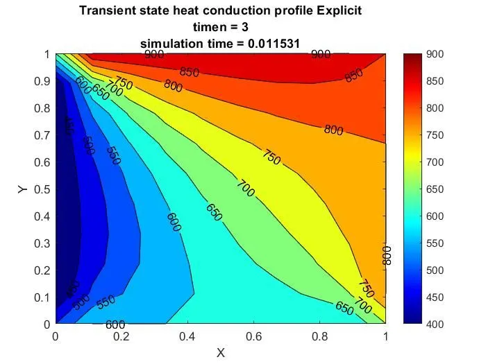
The main advantage of explicit methods is their simplicity and ease of implementation. However, they may be less stable and require smaller time steps to maintain numerical accuracy, especially for stiff differential equations.

1. Implicit Methods: Implicit methods, on the other hand, are numerical techniques that involve solving equations involving unknowns at the next time step in terms of both known and unknown values at the current and/or next time steps. These methods are more involved and often require solving systems of equations, including algebraic or differential equations, to determine the unknown values at the next time step.

One example of an implicit method is the Backward Euler method, used for solving ODEs. The basic formula for the Backward Euler method is:

y_(n+1) = y_n + h * f(t_(n+1), y_(n+1))

In this case, y_(n+1) appears on both sides of the equation, making it an implicit equation. To solve for y_(n+1), one may need to use iterative techniques or more complex numerical algorithms to approximate the solution.

Implicit methods tend to be more stable, even for large time steps, and can handle stiff differential equations better than explicit methods. However, they are usually computationally more expensive and may require more effort to implement.

Code for Transient State Implicitly- 

% Solving Steady and Transient 2D heat conduction problem
% Transient state solution with IMPLICIT
% Iterative solver - Jacobi, Gauss -seidel, Relaxation methods


clear all
close all
clc

%initial conditions
%L = 1
nx = 10;
ny = 10;
nt = 300; % No.of steps
x = linspace(0,1,nx);
y = linspace(0,1,ny);
dx = x(2) - x(1);
dy = y(2) - y(1);


% given data of boundary condition
% initial temp condition

t = 300*ones(nx,ny);  
t(:,1) = 400;
t(1,:) = 600;
t(:,ny) = 800;
t(nx,:) = 900;

% defining the temperature at corner points

t(1,1) = 500;
t(nx,ny) = 850;
t(1,ny) = 700;
t(nx,1) = 650;

dt = 0.01; %time step
told=t;
alpha = 0.3; % Thermal diffusivity
tprev_dt = told;

tol = 1e-4;
k1 = alpha*dt/(dx^2);
k2 = alpha*dt/(dy^2);

method = input('Iterative method = '); %iterative method selection

%JACOBI ITERATIVE METHOD

if (method==1)
    tic;
    jacobi = 1;
    for p = 1:nt
        error =100;
         while(error>tol)
        for i = 2:(nx-1)
            for j = 2:(ny-1)
                term1 = (1+(2*k1)+(2*k2))^-1;
                term2 = k1*term1;
                term3 = k2*term1;
                h = (told(i-1,j)+told(i+1,j));
                v = (told(i,j+1)+told(i,j-1));
                t(i,j) = ((tprev_dt(i,j)*term1)+(h*term2)+(v*term3));
            end
        end
        
    error = max(max(abs(t-told)));
    told = t;
    jacobi = jacobi+1;
         end
         tprev_dt = t ;
    end
    time_taken = toc;

%plotting    
figure(1)
contourf(x,y,t,'ShowText','on');
colormap(jet);
colorbar;
xlabel('X')
ylabel('Y')
text1 = sprintf('number of iteration = %d', jacobi);
text2 = sprintf('simulation time = %f', time_taken);
title({'Transient state heat conduction profile Implicit-Jacobi'; text1; text2});
end


%GAUSS-SEIDEL ITERATIVE METHOD

if (method==2)
    tic;
    gauss = 1;
    for p = 1:nt
        error =100;
         while(error>tol)
        for i = 2:(nx-1)
            for j = 2:(ny-1)
                term1 = (1+(2*k1)+(2*k2))^-1;
                term2 = k1*term1;
                term3 = k2*term1;
                h = (t(i-1,j)+told(i+1,j));
                v = (told(i,j+1)+t(i,j-1));
                t(i,j) = ((tprev_dt(i,j)*term1)+(h*term2)+(v*term3));
            end
        end
        
    error = max(max(abs(t-told)));
    told = t;
    gauss = gauss+1;
         end
         tprev_dt = t; 
    end
    time_taken = toc;

%plotting    
figure(1)
contourf(x,y,t,'ShowText','on');
colormap(jet);
colorbar;
xlabel('X')
ylabel('Y')
text1 = sprintf('number of iteration = %d', gauss);
text2 = sprintf('simulation time = %f', time_taken);
title({'Transient state heat conduction profile Implicit-Gauss-seidel'; text1; text2});
end

%SUCCESSIVE OVER RELAXATION ITERATIVE METHOD

if (method==3)
    tic;
    sor = 1;
    omega = 1.2; % Over relaxation factor
    for p = 1:nt
        error =100;
         while(error>tol)
        for i = 2:(nx-1)
            for j = 2:(ny-1)
                term1 = (1+(2*k1)+(2*k2))^-1;
                term2 = k1*term1;
                term3 = k2*term1;
                h = (t(i-1,j)+told(i+1,j));
                v = (told(i,j+1)+t(i,j-1));
                t(i,j) = (told(i,j)*(1-omega))+(omega*((tprev_dt(i,j)*term1)+(h*term2)+(v*term3)));
            end
        end
        
    error = max(max(abs(t-told)));
    told = t;
    sor = sor+1;
         end
         tprev_dt = t ;
    end
    time_taken = toc;

%plotting    
figure(1)
contourf(x,y,t,'ShowText','on');
colormap(jet);
colorbar;
xlabel('X')
ylabel('Y')
text1 = sprintf('number of iteration = %d', sor);
text2 = sprintf('simulation time = %f', time_taken);
title({'Transient state heat conduction profile Implicit-SOR'; text1; text2});
end

output - 

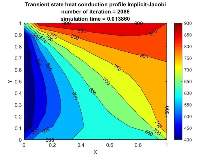
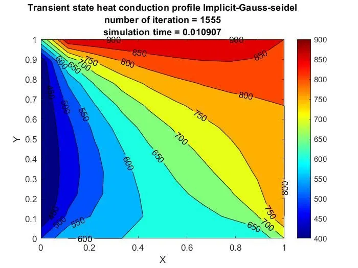
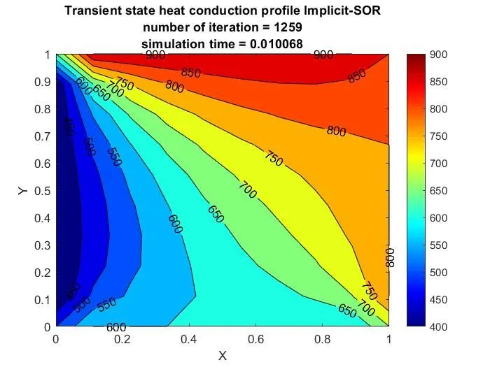
RESULTS AND DISCUSSIONS:

In this study, we compared and discussed the performance of steady state and transient solvers, as well as the efficiency of the Successive Over-Relaxation (SOR) method.

1. Steady State Methods: Steady state methods exhibited faster convergence since they do not involve a time loop. Within just a few iterations, the results reached convergence. As steady state solvers are solely dependent on position and not time, their computational efficiency was significantly higher compared to transient solvers.
2. Transient Solvers: On the other hand, transient solvers required a substantial amount of computation time due to their dependence on both time and position. The inclusion of the time loop in these methods led to a larger number of iterations, resulting in a longer computation time when compared to steady state solvers.
3. Successive Over-Relaxation (SOR) Method: The SOR method demonstrated remarkable efficiency in solving steady-state problems. It provided accurate results with a reduced number of iterations, leading to significant time savings during computations. The introduction of the relaxation factor in the SOR method played a crucial role in accelerating convergence, making it a favourable choice for steady-state simulations.

Conclusion - the choice of solver method depends on the specific requirements of the problem at hand. Steady state methods are ideal when quick convergence is desired, as they eliminate the time loop and converge rapidly with only a few iterations. On the other hand, transient solvers are necessary for problems involving time-dependent phenomena, but they come with increased computation time due to their dependence on both time and position.

For steady state problems, the SOR method emerged as a promising option, providing accurate results with fewer iterations and reduced computation time. Its ability to strike a balance between accuracy and efficiency makes it a valuable tool for various steady-state simulations.

Researchers and engineers should carefully consider the nature of their problem and the trade-offs between accuracy and computation time when selecting the appropriate solver for their simulations.

In your simulation, you observed that explicit methods produced greater accuracy with less computational time required to run them. This outcome is not uncommon, as explicit methods can perform well for certain problems, especially when the stability requirements are met and computational efficiency is critical. However, it is important to note that the choice between explicit and implicit methods depends on various factors, including the specific characteristics of the problem, stability considerations, and available computational resources.

In summary, explicit methods directly compute the next time step values from the current time step, while implicit methods involve solving equations that include future unknowns in terms of current and future knowns. Both approaches have their advantages and disadvantages, and the selection of the most suitable method depends on the specific requirements of the simulation and the nature of the problem being solved.