Week 5.1 - Mid term project - Solving the steady and unsteady 2D heat conduction problem

OBJECTIVE:

1. To perform the Steady State & Transient State Analysis for the 2D heat conduction equation by using the point iterative techniques i.e., Jacobi, Gauss-Seidel, SOR.

Boundary conditions

Top Boundary = 600 K

Bottom Boundary = 900 K

Left Boundary = 400 K

Right Boundary = 800 K

Absolute error criteria are 1e-4.

THEORY:

The 2d heat conduction equation of both stead and transient state of flow. The derivation part where the terms are being discretized sequentially and then we move on to the coding part. There are few things that need to be considered before going over it is that for Steady-state, apply iterative solvers and for Transient, apply schemes IMPLICIT & EXPLICIT.

Since d2t/dx2 + d2T/dy2 = 0, its has elliptic nature properties which we an discretize them using central differencing scheme

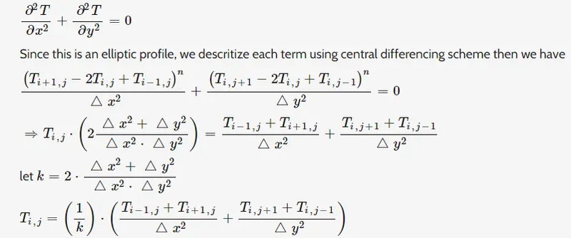
Jacobi:

Gauss Seidel:

SOR (enhanced gauss-seidel method where nth time step and n+1 time step is all same)

where omega is the relaxation factor as 1.4.

now here we begin the coding part which is done in MATLAB where these all terms are considered by applying for loop and while loop.

Explicit & Implicit Methods:

These approaches used in numerical analysis for obtaining numerical approximations to the solutions of time-dependent ordinary and PDEs, as is required in computer simulations of physical process. Explicit methods calculate the state of a system at a later time from the state of the system at the current time, while implicit methods find a solution by solving an equation involving both the current state of the system and the later one. Mathematically, if is the current system state and is the state at the later time is a small time step), then, for an explicit methodwhile for an implicit method one solves an equation

By derivation we have here:

Applying the first heat conduction equation in (1) to node at the time moment of , the equation can be rewritten as

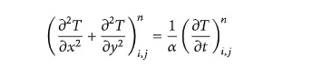
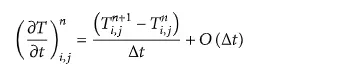
The partial differential in the two sides of (2) can be approximated by difference quotient. The temperature item in the right of the equal sign can be approximated by first-order time forward difference quotient.

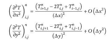
The second-order partial differential in the left of the equal sign can be approximated by the central difference quotient.

Substituting the value, we can get the difference equation of

Equation is the difference equation of heat conduction equation, and the truncation error [34] is O(DT + x2. y2).

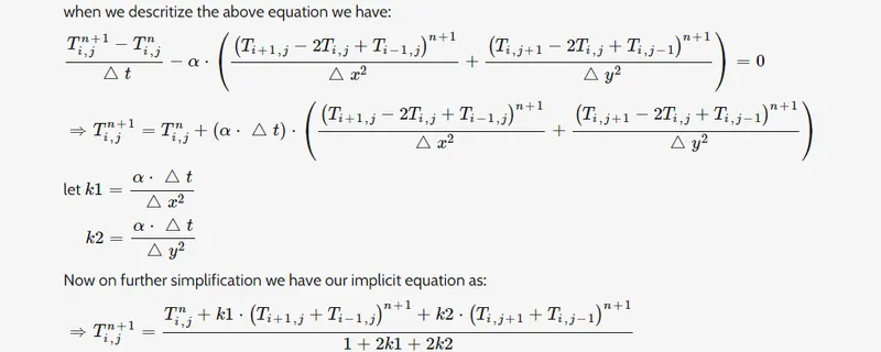
Assuming that deltax = deltay = delta and substituting it into the latest eq., we can obtain

While we discretize the whole equation we get here.

Jacobi:

Gauss-seidel:

Over Relaxation:

CODE FOR STEADY STATE:

% Solving Steady and unsteady 2D heat conduction problem
% Steady state conduction 
% Iterative solver - Jacobi, Gauss -seidel, Relaxation methods

clear all
close all
clc

%initial conditions
%L = 1
nx = 10;
ny = 10;
x = linspace(0,1,nx);
y = linspace(0,1,ny);
dx = x(2) - x(1);
dy = y(2) - y(1);


% given data of boundary condition
% initial temp condition

t = 300*ones(nx,ny);  
t(:,1) = 400;
t(1,:) = 600;
t(:,ny) = 800;
t(nx,:) = 900;

% defining the temperature at corner points

t(1,1) = 500;
t(nx,ny) = 850;
t(1,ny) = 700;
t(nx,1) = 650;

dt = 1e-2; %time step
told=t;

error = 100;
tol = 1e-4;
k = 2*(dx^2+dy^2)/(dx^2*dy^2);
% k2 = (dy^2)/(2*(dx^2+dy^2));

method = input('Iterative method = '); %iterative method selection

%JACOBI ITERATIVE METHOD

if (method==1)
    tic;
    jacobi = 1;
    while(error>tol)
        for i = 2:(nx-1)
            for j = 2:(ny-1)
            t(i,j) = (((told(i-1,j)+told(i+1,j))/(dx^2))+((told(i,j+1)+told(i,j-1))/(dy^2)))/k;
            end
        end
    error = max(max(abs(t-told)));
    told = t;
    jacobi = jacobi+1;
    time_taken = toc;
    end

%plotting    
figure(1)
contourf(x,y,t,'ShowText','on');
colormap(jet);
colorbar;
xlabel('X')
ylabel('Y')
text1 = sprintf('number of iteration = %d', jacobi);
text2 = sprintf('simulation time = %f', time_taken);
title({'Steady state heat condustion profile by jacobi'; text1; text2});
end


%GAUSS-SEIDEL ITERATIVE METHOD

if (method==2)
    tic;
    gauss = 1;
    while(error>tol)
        for i = 2:(nx-1)
            for j = 2:(ny-1)
            t(i,j) = (((t(i-1,j)+told(i+1,j))/(dx^2))+((told(i,j+1)+t(i,j-1))/(dy^2)))/k;
            end
        end
    error = max(max(abs(t-told)));
    told = t;
    gauss = gauss+1;
    time_taken = toc;
    end

%plotting
figure(2)
contourf(x,y,t,'ShowText','on');
colormap(jet);
colorbar;
xlabel('X')
ylabel('Y')
text1 = sprintf('number of iteration = %d', gauss);
text2 = sprintf('simulation time = %f', time_taken);
title({'Steady state heat condustion profile by Gauss-Seidel'; text1; text2});
end


%SUCCESSIVE OVER RELAXATION ITERATIVE METHOD

if (method==3)
    tic;
    sor = 1;
    omega = 1.4; %over relaxation factor
    while(error>tol)
        for i = 2:(nx-1)
            for j = 2:(ny-1)
            term1 =(t(i-1,j)+told(i+1,j))/(dx^2);
            term2 =(told(i,j+1)+t(i,j-1))/(dy^2);
            t(i,j) = ((told(i,j)*(1-omega)))+(omega*(term1+term2))/k;
            end
        end
    error = max(max(abs(t-told)));
    told = t;
    sor = sor+1;
    time_taken = toc;
    end

%plotting
figure(3)
contourf(x,y,t,'ShowText','on');
colormap(jet);
colorbar;
xlabel('X')
ylabel('Y')
text1 = sprintf('number of iteration = %d', sor);
text2 = sprintf('simulation time = %f', time_taken);
text3 = sprintf('over relaxation factor = %f', omega);
title({'Steady state heat condustion profile by Successive Over Relaxation'; text1; text2; text3});
end

OUTPUT FOR STEADY STATE:

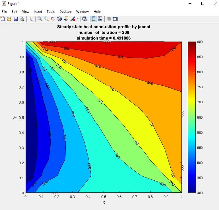
Jacobi Method:

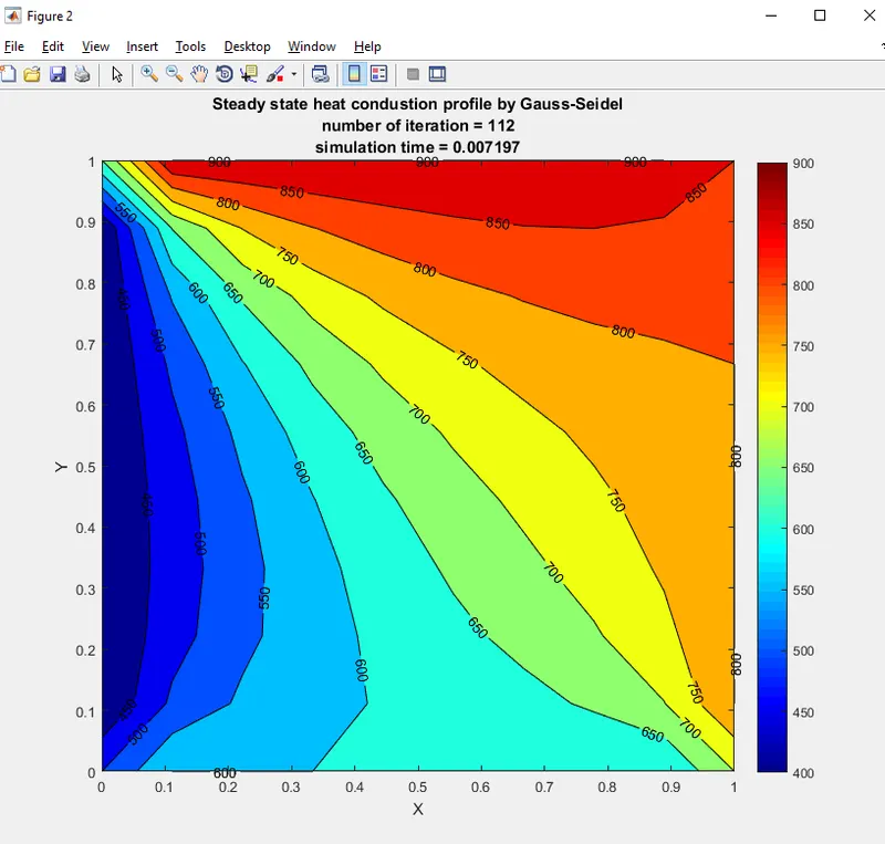
Gauss-seidel Method

SOR Method:

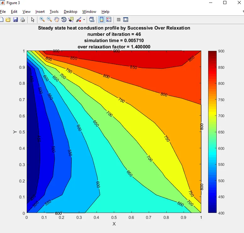
From above results we can see that the SOR method gives a better in terms of iterations carried out by them and no. of simulations time.

CODE FOR TRANSIENT (Unsteady) STATE IMPLICIT:

% Solving Steady and Transient 2D heat conduction problem
% Transient state solution with IMPLICIT
% Iterative solver - Jacobi, Gauss -seidel, Relaxation methods


clear all
close all
clc

%initial conditions
%L = 1
nx = 10;
ny = 10;
nt = 300; % No.of steps
x = linspace(0,1,nx);
y = linspace(0,1,ny);
dx = x(2) - x(1);
dy = y(2) - y(1);


% given data of boundary condition
% initial temp condition

t = 300*ones(nx,ny);  
t(:,1) = 400;
t(1,:) = 600;
t(:,ny) = 800;
t(nx,:) = 900;

% defining the temperature at corner points

t(1,1) = 500;
t(nx,ny) = 850;
t(1,ny) = 700;
t(nx,1) = 650;

dt = 0.01; %time step
told=t;
alpha = 0.3; % Thermal diffusivity
tprev_dt = told;

tol = 1e-4;
k1 = alpha*dt/(dx^2);
k2 = alpha*dt/(dy^2);

method = input('Iterative method = '); %iterative method selection

%JACOBI ITERATIVE METHOD

if (method==1)
    tic;
    jacobi = 1;
    for p = 1:nt
        error =100;
         while(error>tol)
        for i = 2:(nx-1)
            for j = 2:(ny-1)
                term1 = (1+(2*k1)+(2*k2))^-1;
                term2 = k1*term1;
                term3 = k2*term1;
                h = (told(i-1,j)+told(i+1,j));
                v = (told(i,j+1)+told(i,j-1));
                t(i,j) = ((tprev_dt(i,j)*term1)+(h*term2)+(v*term3));
            end
        end
        
    error = max(max(abs(t-told)));
    told = t;
    jacobi = jacobi+1;
         end
         tprev_dt = t ;
    end
    time_taken = toc;

%plotting    
figure(1)
contourf(x,y,t,'ShowText','on');
colormap(jet);
colorbar;
xlabel('X')
ylabel('Y')
text1 = sprintf('number of iteration = %d', jacobi);
text2 = sprintf('simulation time = %f', time_taken);
title({'Transient state heat conduction profile Implicit-Jacobi'; text1; text2});
end


%GAUSS-SEIDEL ITERATIVE METHOD

if (method==2)
    tic;
    gauss = 1;
    for p = 1:nt
        error =100;
         while(error>tol)
        for i = 2:(nx-1)
            for j = 2:(ny-1)
                term1 = (1+(2*k1)+(2*k2))^-1;
                term2 = k1*term1;
                term3 = k2*term1;
                h = (t(i-1,j)+told(i+1,j));
                v = (told(i,j+1)+t(i,j-1));
                t(i,j) = ((tprev_dt(i,j)*term1)+(h*term2)+(v*term3));
            end
        end
        
    error = max(max(abs(t-told)));
    told = t;
    gauss = gauss+1;
         end
         tprev_dt = t; 
    end
    time_taken = toc;

%plotting    
figure(1)
contourf(x,y,t,'ShowText','on');
colormap(jet);
colorbar;
xlabel('X')
ylabel('Y')
text1 = sprintf('number of iteration = %d', gauss);
text2 = sprintf('simulation time = %f', time_taken);
title({'Transient state heat conduction profile Implicit-Gauss-seidel'; text1; text2});
end

%SUCCESSIVE OVER RELAXATION ITERATIVE METHOD

if (method==3)
    tic;
    sor = 1;
    omega = 1.2; % Over relaxation factor
    for p = 1:nt
        error =100;
         while(error>tol)
        for i = 2:(nx-1)
            for j = 2:(ny-1)
                term1 = (1+(2*k1)+(2*k2))^-1;
                term2 = k1*term1;
                term3 = k2*term1;
                h = (t(i-1,j)+told(i+1,j));
                v = (told(i,j+1)+t(i,j-1));
                t(i,j) = (told(i,j)*(1-omega))+(omega*((tprev_dt(i,j)*term1)+(h*term2)+(v*term3)));
            end
        end
        
    error = max(max(abs(t-told)));
    told = t;
    sor = sor+1;
         end
         tprev_dt = t ;
    end
    time_taken = toc;

%plotting    
figure(1)
contourf(x,y,t,'ShowText','on');
colormap(jet);
colorbar;
xlabel('X')
ylabel('Y')
text1 = sprintf('number of iteration = %d', sor);
text2 = sprintf('simulation time = %f', time_taken);
title({'Transient state heat conduction profile Implicit-SOR'; text1; text2});
end

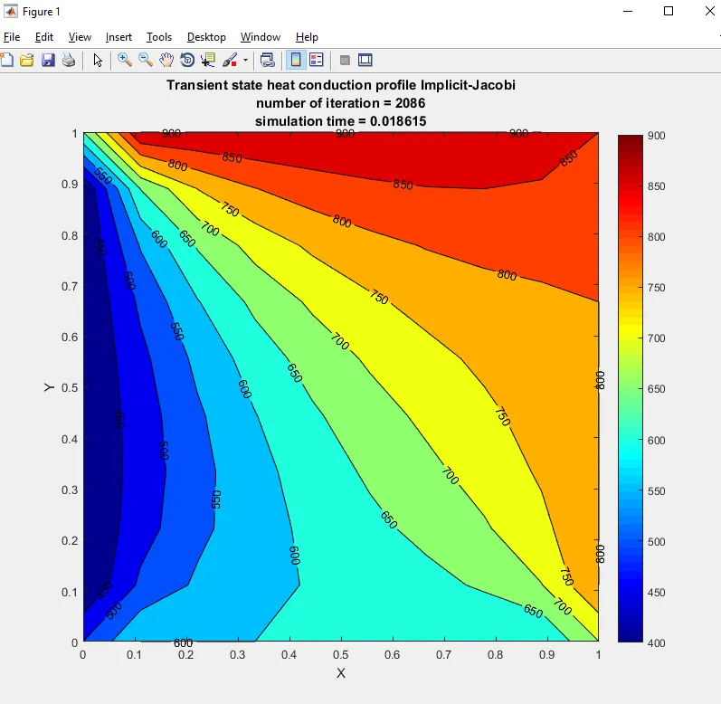
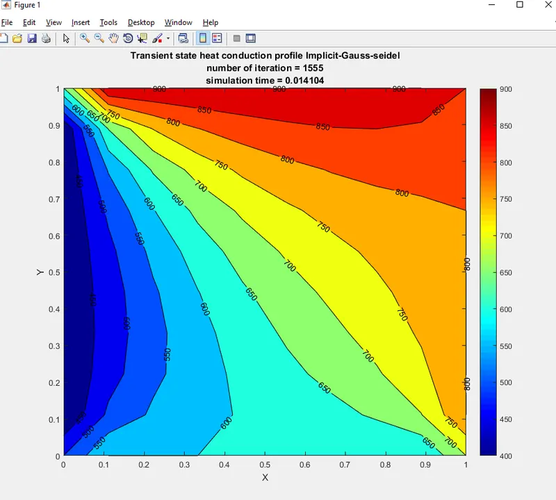
OUTPUT FOR TRANSIENT (Unsteady) STATE IMPLICIT:

Jacobi:

Gauss Seidel:

SOR:

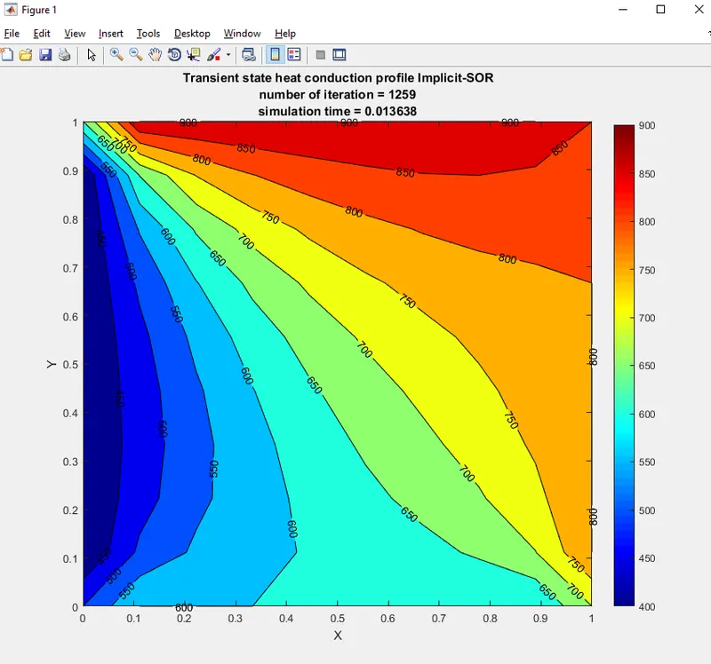
The conclusion of the above results are just as silimar as what was in the steady state, and it was observed that SOR methods gives better results with no. of simulation and time elapsing on the run case.

CODE FOR TRANSIENT (Unsteady) STATE EXPLICIT:

% Solving Steady and Transient 2D heat conduction problem
% Transient state solution with EXPLICIT


clear all
close all
clc

%initial conditions
%L = 1
nx = 10;
ny = 10;
nt = 300; % No.of steps
x = linspace(0,1,nx);
y = linspace(0,1,ny);
dx = x(2) - x(1);
dy = y(2) - y(1);

% initial temp condition

t = 300*ones(nx,ny);  
t(:,1) = 400;
t(1,:) = 600;
t(:,ny) = 800;
t(nx,:) = 900;

% defining the temperature at corner points

t(1,1) = 500;
t(nx,ny) = 850;
t(1,ny) = 700;
t(nx,1) = 650;

dt = 0.01; %time step
told=t;
alpha = 0.3; % Thermal diffusivity

k1 = (alpha*dt)/(dx^2);
k2 = (alpha*dt)/(dy^2);
CFL = alpha*dt/(dx^2);

%EXPLICIT METHOD
% running for loop

tic;
    explicit = 1;
    for p = 1:nt
        for i = 2:(nx-1)
            for j = 2:(ny-1)
                term1 = (told(i-1,j)-2*told(i,j)+told(i+1,j));
                term2 = (told(i,j-1)-2*told(i,j)+told(i,j+1));
                t(i,j) = ((told(i,j))+(k1*term1)+(k2*term2));
            end
        end
        
    told = t;
    explicit = explicit+1;
    end
    
  time_taken = toc; 
  
 %Plotting   
figure(1)
contourf(x,y,t,'ShowText','on');
colormap(jet);
colorbar;
xlabel('X')
ylabel('Y')
text1 = sprintf('timen = %d', dt*nt);
text2 = sprintf('simulation time = %f', time_taken);
title({'Transient state heat conduction profile Explicit'; text1; text2});

OUTPUT FOR TRANSIENT (Unsteady) STATE EXPLICIT:

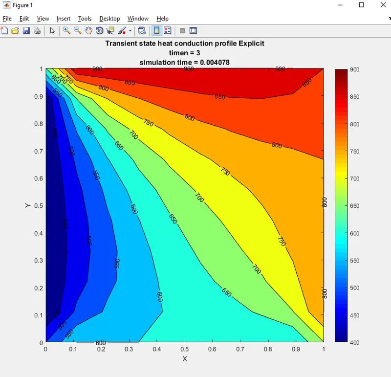
From above simulation we can see explicit method is converging faster than implicit methods taking less time for simulations. For steady state we can opt for SOR method as it reaches converge faster than any other methods.

For explicit methods produce greater accuracy with less computational period require to run it.