Week 5.1 - Mid term project - Solving the steady and unsteady 2D heat conduction problem
Steady State Analysis for 2-D Heat Conduction
For two dimensional steady state,with no heat generation,the Laplace equation applies:
`(d^2T)/(dx^2)+(d^2T)/(dy^2)=0`
`(T(i+1,j)^n-2T(i,j)^n+T(i-1,j)^n)/((dx)^2)+(T(i,j+1)^n-2T(i,j)^n+T(i,j-1)^n)/(dy)^2=0` (Second order central-difference scheme)
`2T(i,j)*[1/(dx)^2+1/(dy)^2]=(T(i+1,j)+T(i-1,j))/((dx)^2)+(T(i,j+1)+T(i,j-1))/(dy)^2`
`2T(i,j)=(dy)^2*[T(i+1,j)+T(i-1,j)]/((dx)^2+(dy)^2)+(dx)^2*[T(i,j+1)+T(i,j-1)]/((dx)^2+(dy)^2`
If dx=dy, `T(i,j)=(T(i+1,j)+T(i-1,j)+T(i,j+1)+T(i,j-1))/4`
Code for Steady-State Analysis
clear all
close all
clc

nx=101;
ny=101;
x=(1:nx)/nx;
y=(1:ny)/ny;

T=675*ones(nx,ny);  %Initial-Condition

%Boundary Conditions------------------------------------------------------
T((2:nx-1),1)=900;
T((2:nx-1),ny)=600;
T(1,(2:ny-1))=400;
T(nx,(2:ny-1))=800;
T(1,1)=650;
T(nx,1)=850;
T(nx,ny)=700;
T(1,ny)=500;
T_old=T;
n=0;

%--------------------------------------------------------------------------


error=1;
while(error>1e-4)
for i=2:nx-1
    for j=2:ny-1
        T(i,j)=0.25*(T_old(i+1,j)+T_old(i-1,j)+T_old(i,j+1)+T_old(i,j-1));
    end
end
error=max(max(abs(T-T_old)));  %Convergence-Criteria
T_old=T;
n=n+1;
end
[X,Y]=meshgrid(x,y);
contourf(Y,X,T,50);
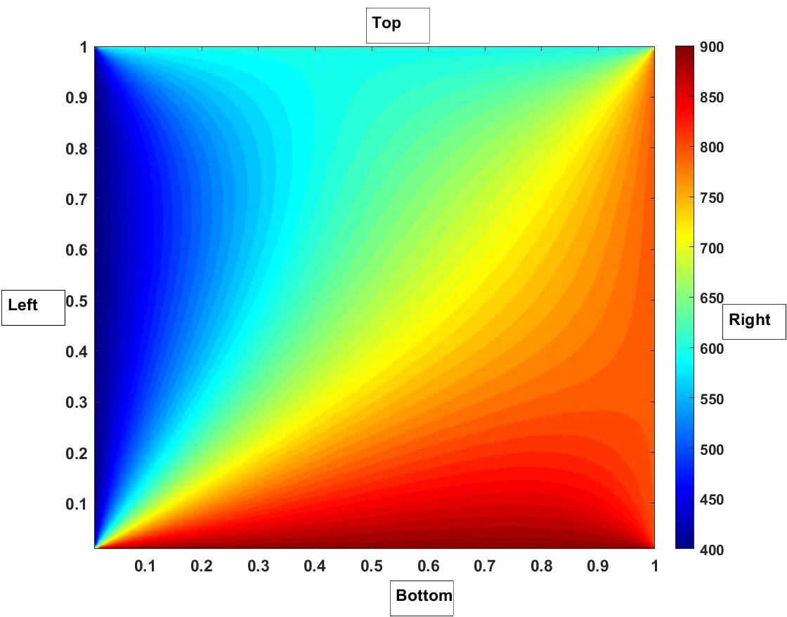
The temperature matrix was initialised by taking the average of the temperature on the four side of the square.The length of the square plate is assumed to be 1.The error criteria was assumed to be 1e-4.If the maximum value of the absolute value of elements of the difference matrix obtained by the difference between the updated and the old temperature matrix falls less than 1e-4,that means that our solution field has achieved the desired converged steady state value.Same is implemented in the code.
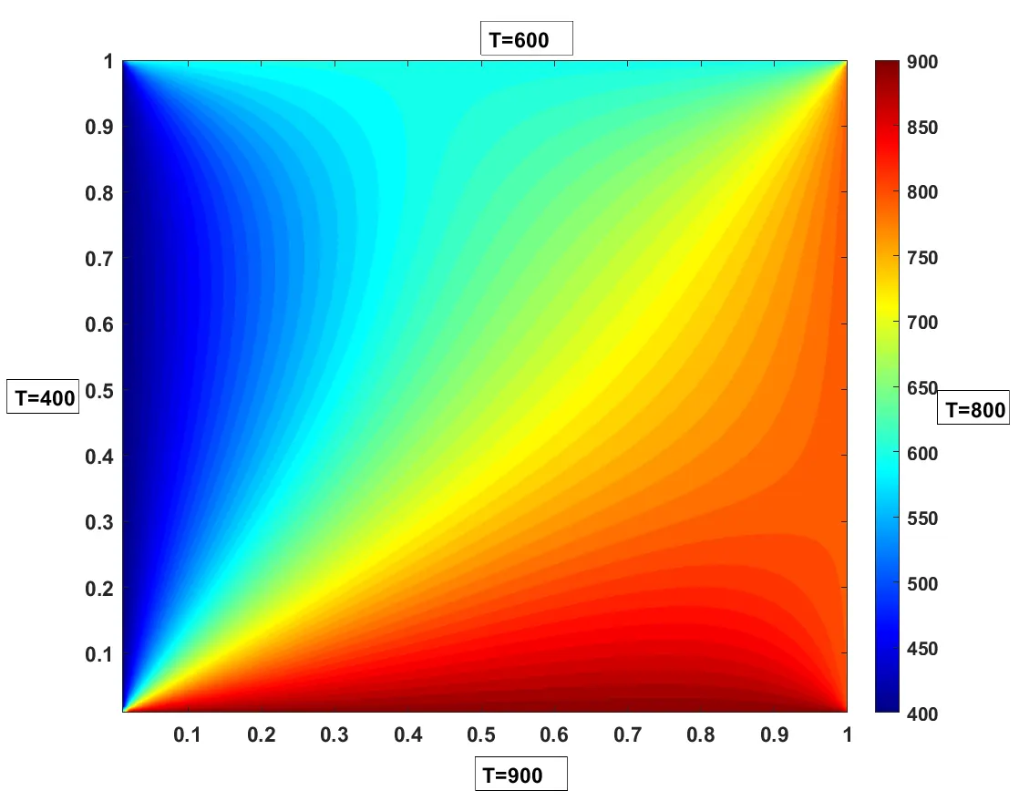
Above picure shows the temperature contours of the solution on the square plate.
`T(i,j)=(T(i+1,j)+T(i-1,j)+T(i,j+1)+T(i,j-1))/4`,As is apparent from the given equation,in a 2D conduction field,the temperature at a point in the
domain depends on the points just neighbouring it and the temperature on the neighbouring points in turn depend on the points neighbouring them.Thus in a 2D conduction field,information from one point effectivvely diffuses to all the points in the domian.Thus we see a continuous temperature field in our solution where the temperature information from the boundaries has uniformly diffused over the entire 2 dimensional domain.
Transient State Analysis:
Explicit Scheme:
`(dT)/(dt)=alpha*((d^2T)/(dx^2)+(d^2T)/dy^2)`
`(T^(n+1)-T^n)/dt=alpha/(dx)^2*(T^n(i+1,j)-2T^n(i,j)+T^n(i-1,j))+alpha/(dy)^2*(T^n(i,j+1)-2T^n(i,j)+T(i,j-1)^n)`
`T^(n+1)=T^n+(alphadt)/(dx)^2*(T^n(i+1,j)-2T^n(i,j)+T^n(i-1,j))+(alphadt)/(dy)^2*(T^n(i,j+1)-2T^n(i,j)+T(i,j-1)^n)`
Code for the Explicit Scheme:
clear all
close all
clc

nx=101;
ny=101;
x=(1:nx)/nx;
y=(1:ny)/ny;
dx=1/(nx-1);
dy=1/(ny-1);
dt=2e-5;
alpha=1.2;

T=675*ones(nx,ny); %Initializing the temperature field

%Boundary Conditions------------------------------------------------------
T((2:nx-1),1)=900;
T((2:nx-1),ny)=600;
T(1,(2:ny-1))=400;
T(nx,(2:ny-1))=800;
T(1,1)=650;
T(nx,1)=850;
T(nx,ny)=700;
T(1,ny)=500;
T_old=T;
n=0;
CFL_x=alpha*dt/(dx*dx);
CFL_y=alpha*dt/(dy*dy);
error=1;
nt=10000;         %No of time steps


      for i=1:nt
        for i=2:nx-1
            for j=2:ny-1
                T(i,j)=(T_old(i+1,j)-2*T_old(i,j)+T_old(i-1,j))*CFL_x+(T_old(i,j+1)-2*T_old(i,j)+T_old(i,j-1))*CFL_y+T_old(i,j);

            end
        end


       error=max(max(abs(T-T_old)));
       disp(error);
       T_old=T;            %Updating th Temperature field


        n=n+1;
end
    [X,Y]=meshgrid(x,y);
contourf(Y,X,T,50);
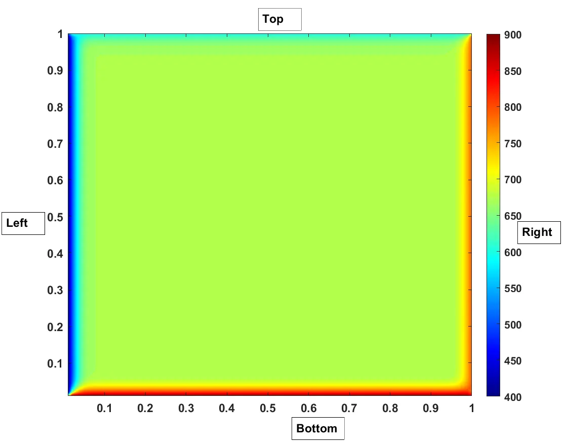
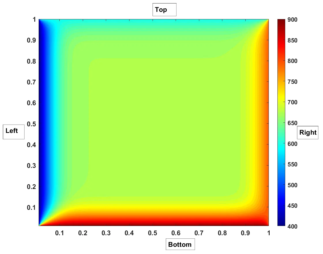
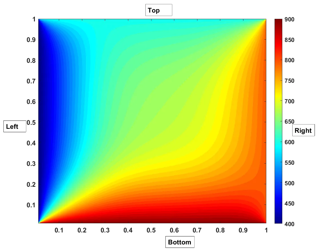
Results for the transient analysis using the Explicit Scheme:
Solution for t=2e-4 s:
Solution for t=2e-3 s:
Solution for t=2e-2 s:
Solution for t=0.2 secs:
Implicit Method for transient Analysis:
`(dT)/(dt)=alpha*((d^2T)/(dx^2)+(d^2T)/(dy^2))`
`(T(i,j)^(n+1)-T(i,j)^(n))/dt=(alpha)/(dx)^2*(T(i+1,j)^(n+1)-2T(i,j)^(n+1)+T(i-1,j)^(n+1))+(alpha)/(dy)^2*(T(i,j+1)^(n+1)-2T(i,j)^(n+1)+T(i,j-1)^(n+1)`
`T(i,j)^(n+1)-T(i,j)^n=(alphadt)/(dx)^2*(T(i+1,j)^(n+1)-2T(i,j)^(n+1)+T(i-1,j)^(n+1))+(alphadt)/(dy)^2*(T(i,j+1)^(n+1)-2T(i,j)^(n+1)+T(i,j-1)^(n+1))`
On rearranging the terms,we get:
`T(i,j)^(n+1)*(1+(2alphadt)/(dx)^2+(2alphadt)/(dy)^2)=T(i,j)^n+(alphadt)/(dx)^2*(T(i+1,j)^(n+1)+T(i-1,j)^(n+1))+(alphadt)/(dy)^2*(T(i,j+1)^(n+1)+T(i,j-1)^(n+1))`
k1=`(1+(2alphadt)/(dx)^2+(2alphadt)/(dy)^2)`
CFL_X=`(alphadt)/(dx)^2`
CFL_Y=`(alphadt)/(dy)^2`
k2=CFL_X/k1;
k3=CFL_Y/k1;
The final expression comes out to be:
`T(i,j)^(n+1)=(T(i,j)^(n))/(k1)+k2*(T(i+1,j)^(n+1)+T(i-1,j)^(n+1))+k3*(T(i,j+1)^(n+1)+T(i,j-1)^(n+1))`
a) Jacobi Method
clear all
close all
clc

nx=101;
ny=101;
x=(1:nx)/nx;
y=(1:ny)/ny;
dx=1/(nx-1);
dy=1/(ny-1);
dt=1;
alpha=1.2;

T=675*ones(nx,ny); %Initializing temperature field

%Boundary Conditions------------------------------------------------------
T((2:nx-1),1)=900;
T((2:nx-1),ny)=600;
T(1,(2:ny-1))=400;
T(nx,(2:ny-1))=800;
T(1,1)=650;
T(nx,1)=850;
T(nx,ny)=700;
T(1,ny)=500;

n1=0;
n2=0;
error1=1;
error2=1;
CFL_x=alpha*dt/(dx*dx);
CFL_y=alpha*dt/(dy*dy);
k1=(1+2*CFL_x+2*CFL_y);
k2=CFL_x/k1;
k3=CFL_y/k1;


error1=1;
error2=1;
T_current_old=T;  %Initialising the variables
T_previous=T;
T_current=T;
w=1.5;
while(error2>1e-5)  %Time-Loop
    T_previous=T_current;
while (error1>1e-5)  %Space loop at a particular instant
    T_current_old=T_current;
for i=2:nx-1
    for j=2:ny-1
     T_current(i,j)=(T_previous(i,j)/k1+k2*(T_current_old(i+1,j)+T_current_old(i-1,j))+k3*(T_current_old(i,j+1)+T_current_old(i,j-1)));

    end
end
error1=max(max(abs(T_current-T_current_old)));
%disp(error1);

n1=n1+1;
end
error2=max(max(abs(T_current-T_previous)));
disp(error2);
n2=n2+1;
end
[X,Y]=meshgrid(x,y);
contourf(Y,X,T_current,50);
In the Jacobi method,values of the temperature calculated in the k'th iteration reamains entirely unchanged till the values of the temperature in the (k+1)'th iteration have been calculated.
The solution reaches the steady state value just after two iterations of the time loop for nx=101,ny=101,dt=1.For each time iteration the code has taken 7956 iterations to reach convergence.
Solution:
b)Gauss-Seidel Method:
Code for Gauss-Seidel:
clear all
close all
clc

nx=101;
ny=101;
x=(1:nx)/nx;
y=(1:ny)/ny;
dx=1/(nx-1);
dy=1/(ny-1);
dt=1;
alpha=1.2;

T=675*ones(nx,ny);   %Initialising temperature field

%Boundary Conditions------------------------------------------------------
T((2:nx-1),1)=900;
T((2:nx-1),ny)=600;
T(1,(2:ny-1))=400;
T(nx,(2:ny-1))=800;
T(1,1)=650;
T(nx,1)=850;
T(nx,ny)=700;
T(1,ny)=500;

n1=0;
n2=0;
error1=ones(500,1);
error2=ones(500,1);
CFL_x=alpha*dt/(dx*dx);
CFL_y=alpha*dt/(dy*dy);

k1=(1+2*CFL_x+2*CFL_y);
k2=CFL_x/k1;
k3=CFL_x/k1;
error=1;
T_current_old=T;
T_previous=T;
T_current=T;
w=1.2;
while (error2>1e-5) %Time-Loop
    T_previous=T_current;
while (error1>1e-5) %Space-Loop
    T_current_old=T_current;
for i=2:nx-1
    for j=2:ny-1
     T_current(i,j)=(T_previous(i,j)/k1+k2*(T_current(i+1,j)+T_current(i-1,j))+k3*(T_current(i,j+1)+T_current(i,j-1)));

    end
end
%T_current(i,j)=(1-w)*T_previous(i,j)+w*(T_current(i,j));
error1=max(max(abs(T_current-T_current_old)));
%disp(error1);

n1=n1+1;
end
error2=max(max(abs(T_current-T_previous)));
disp(n1);
disp(error2);
n2=n2+1;
end
[X,Y]=meshgrid(x,y);
contourf(Y,X,T_current,50);
Here too,the Gauss-Seidel method achieves steady state values in two time steps.The method achieves convergence faster compared to the Jacobi method.
As opposed to Jacobi Method,the Gauss-Seidel method uses the value of (k+1)th iteration as soon as they are know.Gauss-Seidel achieve convergence faster compared to Jacobi method.
Solution:
c)Gauss-Seidel Succesive over relaxation:
Even though the successive over relaxation technique is used to achieve faster convergence,in this case,no difference could be established
between the methods in terms of total number of iterations required for convergence.
Code:
clear all
close all
clc

nx=101;
ny=101;
x=(1:nx)/nx;
y=(1:ny)/ny;
dx=1/(nx-1);
dy=1/(ny-1);
dt=1;
alpha=1.2;

T=675*ones(nx,ny);   %Initialising temperature field

%Boundary Conditions------------------------------------------------------
T((2:nx-1),1)=900;
T((2:nx-1),ny)=600;
T(1,(2:ny-1))=400;
T(nx,(2:ny-1))=800;
T(1,1)=650;
T(nx,1)=850;
T(nx,ny)=700;
T(1,ny)=500;

n1=0;
n2=0;
error1=ones(500,1);
error2=ones(500,1);
CFL_x=alpha*dt/(dx*dx);
CFL_y=alpha*dt/(dy*dy);

k1=(1+2*CFL_x+2*CFL_y);
k2=CFL_x/k1;
k3=CFL_x/k1;
error=1;
T_current_old=T;
T_previous=T;
T_current=T;
w=1.2;
while (error2>1e-5) %Time-Loop
    T_previous=T_current;
while (error1>1e-5) %Space-Loop
    T_current_old=T_current;
for i=2:nx-1
    for j=2:ny-1
     T_current(i,j)=(T_previous(i,j)/k1+k2*(T_current(i+1,j)+T_current(i-1,j))+k3*(T_current(i,j+1)+T_current(i,j-1)));

    end
end
%T_current(i,j)=(1-w)*T_previous(i,j)+w*(T_current(i,j)); %Successive over-relaxation
error1=max(max(abs(T_current-T_current_old)));
%disp(error1);

n1=n1+1;
end
error2=max(max(abs(T_current-T_previous)));
disp(n1);
disp(error2);
n2=n2+1;
end
[X,Y]=meshgrid(x,y);
contourf(Y,X,T_current,50);
Here too,steady state solution was achieved in two time steps.
Solution: