Week 5.1 - Mid term project - Solving the steady and unsteady 2D heat conduction problem
PROBLEM STAEMENT:-
- Steady state analysis & Transient State Analysis
Solve the 2D heat conduction equation by using the point iterative techniques that were taught in the class. The Boundary conditions for the problem are as follows;
Top Boundary = 600 K
Bottom Boundary = 900 K
Left Boundary = 400 K
Right Boundary = 800 K
You will implement the following methods for solving implicit equations.
- Jacobi
- Gauss-seidel
- Successive over-relaxation
Your absolute error criteria is 1e-4
Objective:
The objective of this code is to solve the steady-state and unsteady 2D heat conduction equations using point iterative techniques, specifically the Jacobi method and the Gauss-Seidel method. The code will take as input the necessary parameters, including the number of grid points, domain size, boundary conditions, and time step size (for the unsteady case). The code will then solve the heat conduction equations using the iterative methods until the desired level of accuracy is achieved, and the temperature distribution will be plotted.
Theory:
The steady-state and unsteady 2D heat conduction equations are given by:
Steady-state: d^2T/dx^2 + d^2T/dy^2 = 0
Unsteady: dT/dt = alpha*(d^2T/dx^2 + d^2T/dy^2)
where T is the temperature, x and y are the spatial coordinates, t is the time, and alpha is the thermal diffusivity of the material.
To solve these equations numerically, the domain is discretized into a grid, and the temperature at each grid point is approximated using a finite difference approximation. The point iterative techniques, such as the Jacobi method and the Gauss-Seidel method, are then used to iteratively solve the discretized equations until the desired level of accuracy is achieved.
In the Jacobi method, the temperature at each grid point is updated using the previous iteration values at all grid points. In the Gauss-Seidel method, the temperature at each grid point is updated using the previous iteration values at the neighboring grid points, which can result in faster convergence than the Jacobi method.
For the unsteady case, the time integration is performed using the Forward Euler method, which approximates the time derivative using a first-order finite difference approximation. The unsteady heat conduction equation is then discretized using a combination of finite difference approximations in space and time, and the point iterative techniques are used to iteratively solve the resulting system of equations at each time step until the desired level of accuracy is achieved.
Once the iterative solution is obtained, the temperature distribution is plotted using MATLAB's contourf function, and the results are analyzed to ensure accuracy and validity.
SOLUTION:-
Jacobi Iteration
close all
clear all
clc

%Solving the Steady state 2D heat conduction (Jacobi Method)

%Input Parameters
%Number of grid points
nx = 10;
ny = nx;

x = linspace(0,1,nx);
y = linspace(0,1,ny);

dx = x(2) - x(1);
dy = dx;

%Absolute error criteria > tolerance
error = 9e9;
tolerance = 1e-4;

%Defining Boundary conditions
T_L = 400;
T_T = 600;
T_R = 800;
T_B = 900;

T = 300*ones(nx,ny);

T(2:ny - 1, 1)  = T_L;
T(2:ny - 1, nx) = T_R;
T(1, 2:nx - 1)  = T_T;
T(ny, 2:nx - 1) = T_B;

%Calculating Average temperature at corners
T(1,1) = (T_T + T_L)/2;
T(nx,ny) = (T_R + T_B)/2;
T(1,ny) = (T_T + T_R)/2;
T(nx,1) = (T_L + T_B)/2;

%Assigning orginal values to T
T_intial = T;
T_old = T;


%Calculation of 2D steady heat conduction EQUATION by JACOBI method
iterative_solver = 1;

if iterative_solver == 1
    jacobi_iteration = 1;

    while(error > tolerance)

        for i = 2:nx - 1

            for j = 2:ny - 1
                T(i,j) = 0.25*(T_old(i-1,j) + T_old(i+1,j) + T_old(i,j-1) + T_old(i,j+1));
            end

        end

        error = max(max(abs(T_old - T)));
        T_old = T;
        jacobi_iteration = jacobi_iteration + 1;

    end
end

%Plotting
figure(1)
contourf(x,y,T)
clabel(contourf(x,y,T))
colorbar
colormap(jet)
set(gca, 'ydir', 'reverse')

xlabel('X-Axis')
ylabel('Y-Axis')
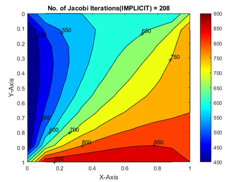
title(sprintf('No. of Jacobi Iterations(IMPLICIT) = %d', jacobi_iteration));
pause(0.03);
Output
Gauss-Siedel Iteration
close all
clear all
clc

%Solving the Steady state 2D heat conduction (Gauss-seidel Method)

%Input Parameters
%Number of grid points
nx = 10;
ny = nx;

x = linspace(0,1,nx);
y = linspace(0,1,ny);

dx = x(2) - x(1);
dy = dx;

%Absolute error criteria > tolerance
error = 9e9;
tolerance = 1e-4;

%Defining Boundary conditions
T_L = 400;
T_T = 600;
T_R = 800;
T_B = 900;

T = 300*ones(nx,ny);

T(2:ny - 1, 1)  = T_L;
T(2:ny - 1, nx) = T_R;
T(1, 2:nx - 1)  = T_T;
T(ny, 2:nx - 1) = T_B;

%Calculating Average temperature at corners
T(1,1) = (T_T + T_L)/2;
T(nx,ny) = (T_R + T_B)/2;
T(1,ny) = (T_T + T_R)/2;
T(nx,1) = (T_L + T_B)/2;

%Assigning orginal values to T
T_intial = T;
T_old = T;


%Calculation of 2D steady heat conduction EQUATION by Gauss-Seidel method
iterative_solver = 2;

if iterative_solver == 2
    Gauss_seidel_iteration = 1;

    while(error > tolerance)

        for i = 2:nx - 1

            for j = 2:ny - 1
                T(i,j) = 0.25*(T(i-1,j) + T_old(i+1,j) + T(i,j-1) + T_old(i,j+1));
            end

        end

        error = max(max(abs(T_old - T)));
        T_old = T;
        Gauss_seidel_iteration = Gauss_seidel_iteration + 1;

    end
end

%Plotting
figure(1)
contourf(x,y,T)
clabel(contourf(x,y,T))
colorbar
colormap(jet)
set(gca, 'ydir', 'reverse')

xlabel('X-Axis')
ylabel('Y-Axis')
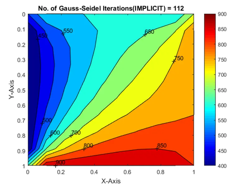
title(sprintf('No. of Gauss-Seidel Iterations(IMPLICIT) = %d', Gauss_seidel_iteration));
pause(0.03);
Output
Successive over-relaxation
close all
clear all
clc

%Solving the Steady state 2D heat conduction (Successive over-relaxation Method)

%Input Parameters
%Number of grid points
nx = 10;
ny = nx;

x = linspace(0,1,nx);
y = linspace(0,1,ny);

dx = x(2) - x(1);
dy = dx;

%Absolute error criteria > tolerance
error = 9e9;
tolerance = 1e-4;
omega = 1.2;

%Defining Boundary conditions
T_L = 400;
T_T = 600;
T_R = 800;
T_B = 900;

T = 300*ones(nx,ny);

T(2:ny - 1, 1)  = T_L;
T(2:ny - 1, nx) = T_R;
T(1, 2:nx - 1)  = T_T;
T(ny, 2:nx - 1) = T_B;

%Calculating Average temperature at corners
T(1,1) = (T_T + T_L)/2;
T(nx,ny) = (T_R + T_B)/2;
T(1,ny) = (T_T + T_R)/2;
T(nx,1) = (T_L + T_B)/2;

%Assigning orginal values to T
T_intial = T;
T_old = T;


%Calculation of 2D steady heat conduction EQUATION by Successive over-relaxation method
iterative_solver = 3;

if iterative_solver == 3
    Successive_Over_Relaxation_iteration = 1;

    while(error > tolerance)

        for i = 2:nx - 1

            for j = 2:ny - 1
                T(i,j) = omega*(0.25*(T(i-1,j) + T_old(i+1,j) + T(i,j-1) + T_old(i,j+1))) + (1 - omega)*T_old(i,j);
            end

        end

        error = max(max(abs(T_old - T)));
        T_old = T;
        Successive_Over_Relaxation_iteration = Successive_Over_Relaxation_iteration + 1;

    end
end

%Plotting
figure(1)
contourf(x,y,T)
clabel(contourf(x,y,T))
colorbar
colormap(jet)
set(gca, 'ydir', 'reverse')

xlabel('X-Axis')
ylabel('Y-Axis')
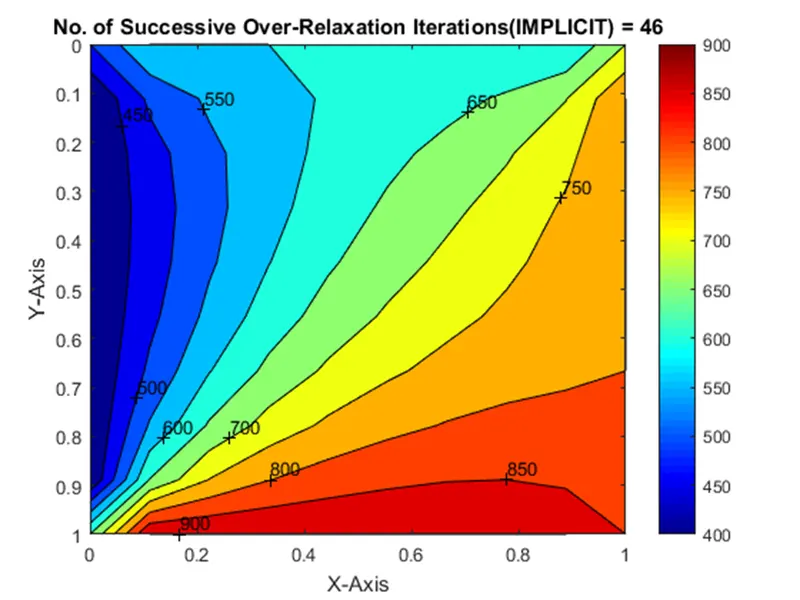
title(sprintf('No. of Successive Over-Relaxation Iterations(IMPLICIT) = %d', Successive_Over_Relaxation_iteration));
pause(0.03);
Output
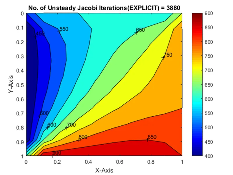
IMPLICIT Scheme Unsteady/Transient-state Condition Program:
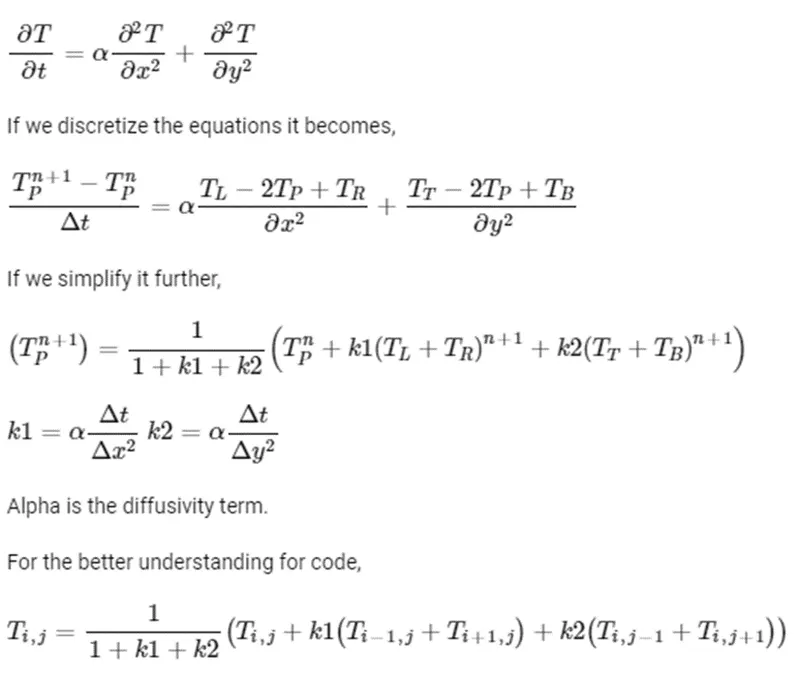
Unsteady-state Equation discretization:
Non-steady-state situations appear after an imposed change in temperature at a boundary as well as inside of an object, as a result of a new source or sink of heat suddenly introduced within an object, causing temperatures near the source or sink to change in time.
Jacobi Iteration
close all
clear all
clc

%Solving the Unsteady state 2D heat conduction by Jacobi Method(IMPLICIT SCHEME)

%Input Parameters
%Number of grid points
nx = 10;
ny = nx;
nt = 1400;

x = linspace(0,1,nx);
y = linspace(0,1,ny);

dx = x(2) - x(1);
dy = dx;

%Absolute error criteria > tolerance
error = 9e9;
tolerance = 1e-4;
dt = 1e-3;

%Defining Boundary conditions
T_L = 400;
T_T = 600;
T_R = 800;
T_B = 900;

T = 300*ones(nx,ny);

T(2:ny - 1, 1)  = T_L;
T(2:ny - 1, nx) = T_R;
T(1, 2:nx - 1)  = T_T;
T(ny, 2:nx - 1) = T_B;

%Calculating Average temperature at corners
T(1,1) = (T_T + T_L)/2;
T(nx,ny) = (T_R + T_B)/2;
T(1,ny) = (T_T + T_R)/2;
T(nx,1) = (T_L + T_B)/2;

%Assigning orginal values to T
T_old = T;
T_intial = T;

%Calculation of 2D steady heat conduction EQUATION by Successive over-relaxation method
k1 = 1.1*(dt/(dx^2));
k2 = 1.1*(dt/(dy^2));

Jacobi_iteration = 1;
for k = 1:nt
    error = 9e9;

    while(error > tolerance)

        for i = 2:nx - 1

            for j = 2:ny - 1

                Term_1 = 1/(1 + (2*k1) + (2*k2));
                Term_2 = k1*Term_1;
                Term_3 = k2*Term_1;
                H = (T_old(i-1,j)) + (T_old(i+1,j));
                V = (T_old(i,j+1)) + (T_old(i,j-1));

                T(i,j) = (T_intial(i,j)*Term_1) + (H*Term_2) + (V*Term_3);

            end

        end

        error = max(max(abs(T_old - T)));
        T_old = T;
        Jacobi_iteration = Jacobi_iteration + 1;

    end

    T_intial = T;

    %Plotting
    figure(1)
    contourf(x,y,T)
    clabel(contourf(x,y,T))
    colorbar
    colormap(jet)
    set(gca, 'ydir', 'reverse')

    xlabel('X-Axis')
    ylabel('Y-Axis')
    title(sprintf('No. of Unsteady Jacobi Iterations(EXPLICIT) = %d', Jacobi_iteration));
    pause(0.03)
end
Output
Gauss-Siedel Iteration
close all
clear all
clc

%Solving the Unsteady state 2D heat conduction by Gauss Seidel Method(IMPLICIT SCHEME)

%Input Parameters
%Number of grid points
nx = 10;
ny = nx;
nt = 1400;

x = linspace(0,1,nx);
y = linspace(0,1,ny);

dx = x(2) - x(1);
dy = dx;

%Absolute error criteria > tolerance
error = 9e9;
tolerance = 1e-4;
dt = 1e-3;

%Defining Boundary conditions
T_L = 400;
T_T = 600;
T_R = 800;
T_B = 900;

T = 300*ones(nx,ny);

T(2:ny - 1, 1)  = T_L;
T(2:ny - 1, nx) = T_R;
T(1, 2:nx - 1)  = T_T;
T(ny, 2:nx - 1) = T_B;

%Calculating Average temperature at corners
T(1,1) = (T_T + T_L)/2;
T(nx,ny) = (T_R + T_B)/2;
T(1,ny) = (T_T + T_R)/2;
T(nx,1) = (T_L + T_B)/2;

%Assigning orginal values to T
T_old = T;
T_intial = T;

%Calculation of 2D steady heat conduction EQUATION by Successive over-relaxation method
k1 = 1.1*(dt/(dx^2));
k2 = 1.1*(dt/(dy^2));

Gauss_Seidel_iteration = 1;
for k = 1:nt
    error = 9e9;

    while(error > tolerance)

        for i = 2:nx - 1

            for j = 2:ny - 1

                Term_1 = 1/(1 + (2*k1) + (2*k2));
                Term_2 = k1*Term_1;
                Term_3 = k2*Term_1;
                H = (T(i-1,j)) + (T_old(i+1,j));
                V = (T(i,j+1)) + (T_old(i,j-1));

                T(i,j) = (T_intial(i,j)*Term_1) + (H*Term_2) + (V*Term_3);

            end

        end

        error = max(max(abs(T_old - T)));
        T_old = T;
        Gauss_Seidel_iteration = Gauss_Seidel_iteration + 1;

    end

    T_intial = T;

    %Plotting
    figure(1)
    contourf(x,y,T)
    clabel(contourf(x,y,T))
    colorbar
    colormap(jet)
    set(gca, 'ydir', 'reverse')

    xlabel('X-Axis')
    ylabel('Y-Axis')
    title(sprintf('No. of Unsteady Gauss-Seidel Iterations(IMPLICIT) = %d', Gauss_Seidel_iteration));
    pause(0.03)
end
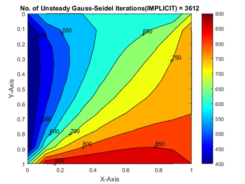
Output
Successive over-relaxation
close all
clear all
clc

%Solving the Unsteady state 2D heat conduction by Successive over-relaxation Method(IMPLICIT SCHEME)

%Input Parameters
%Number of grid points
nx = 10;
ny = nx;
nt = 1400;

x = linspace(0,1,nx);
y = linspace(0,1,ny);

dx = x(2) - x(1);
dy = dx;

%Absolute error criteria > tolerance
error = 9e9;
tolerance = 1e-4;
dt = 1e-3;
omega = 1.1;

%Defining Boundary conditions
T_L = 400;
T_T = 600;
T_R = 800;
T_B = 900;

T = 300*ones(nx,ny);

T(2:ny - 1, 1)  = T_L;
T(2:ny - 1, nx) = T_R;
T(1, 2:nx - 1)  = T_T;
T(ny, 2:nx - 1) = T_B;

%Calculating Average temperature at corners
T(1,1) = (T_T + T_L)/2;
T(nx,ny) = (T_R + T_B)/2;
T(1,ny) = (T_T + T_R)/2;
T(nx,1) = (T_L + T_B)/2;

%Assigning orginal values to T
T_old = T;
T_intial = T;
T_end = T;

%Calculation of 2D steady heat conduction EQUATION by Successive over-relaxation method
k1 = 1.1*(dt/(dx^2));
k2 = 1.1*(dt/(dy^2));

Successive_over_relaxation_iteration = 1;
for k = 1:nt
    error = 9e9;

    while(error > tolerance)

        for i = 2:nx - 1

            for j = 2:ny - 1

                Term_1 = 1/(1 + (2*k1) + (2*k2));
                Term_2 = k1*Term_1;
                Term_3 = k2*Term_1;
                H = (T(i-1,j)) + (T_old(i+1,j));
                V = (T(i,j+1)) + (T_old(i,j-1));

                T(i,j) = (T_intial(i,j)*Term_1) + (H*Term_2) + (V*Term_3);
                T_end(i,j) = ((1-omega)*T_old(i,j)) + (T(i,j)*omega);

            end

        end

        error = max(max(abs(T_old - T)));
        T_old = T_end;
        Successive_over_relaxation_iteration = Successive_over_relaxation_iteration + 1;

    end

    T_intial = T_end;

    %Plotting
    figure(1)
    contourf(x,y,T)
    clabel(contourf(x,y,T))
    colorbar
    colormap(jet)
    set(gca, 'ydir', 'reverse')

    xlabel('X-Axis')
    ylabel('Y-Axis')
    title(sprintf('No. of Unsteady SOR Iterations(IMPLICIT) = %d', Successive_over_relaxation_iteration));
    pause(0.03)
end
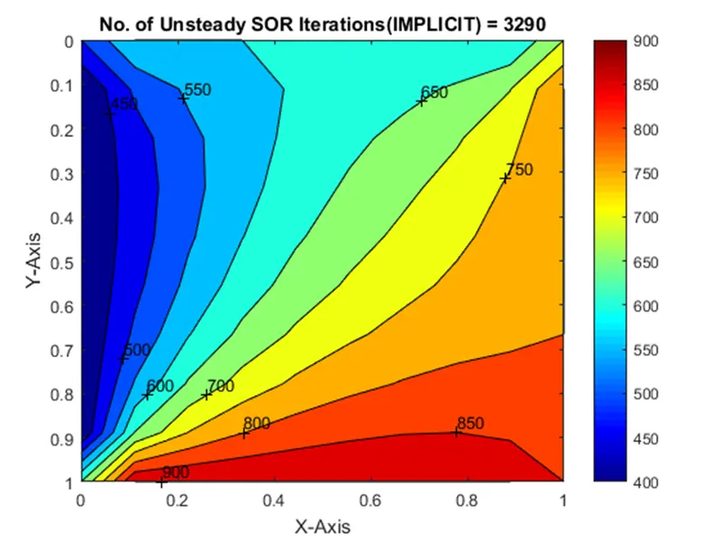
Output
EXPLICIT Scheme - Unsteady/Transient state Condition Program
close all
clear all
clc

%Solving the Unsteady state 2D heat conduction (EXPLICIT SCHEME)

%Input Parameters
%Number of grid points
nx = 10;
ny = nx;
nt = 1400;

x = linspace(0,1,nx);
y = linspace(0,1,ny);

dx = x(2) - x(1);
dy = dx;

%Absolute error criteria > tolerance
error = 9e9;
tolerance = 1e-4;
dt = 1e-3;
omega = 1.1;

%Defining Boundary conditions
T_L = 400;
T_T = 600;
T_R = 800;
T_B = 900;

T = 300*ones(nx,ny);

T(2:ny - 1, 1)  = T_L;
T(2:ny - 1, nx) = T_R;
T(1, 2:nx - 1)  = T_T;
T(ny, 2:nx - 1) = T_B;

%Calculating Average temperature at corners
T(1,1) = (T_T + T_L)/2;
T(nx,ny) = (T_R + T_B)/2;
T(1,ny) = (T_T + T_R)/2;
T(nx,1) = (T_L + T_B)/2;

%Assigning orginal values to T
T_intial = T;
T_old = T;


%Calculation of 2D steady heat conduction EQUATION by Successive over-relaxation method
iterative_solver = 1;
k1 = 1.1*(dt/(dx^2));
k2 = 1.1*(dt/(dy^2));

if iterative_solver == 1
    Steady_Explicit = 1;
    for k = 1:nt
        error = 1;

        while(error > tolerance)

            for i = 2:nx - 1

                for j = 2:ny - 1
                    Term_1 = T_old(i,j);
                    Term_2 = k1*(T_old(i+1,j) - 2*T_old(i,j) + (T_old(i-1,j)));
                    Term_3 = k2*(T_old(i,j+1) - 2*T_old(i,j) + T_old(i,j-1));
                    T(i,j) = Term_1 + Term_2 + Term_3;
                end

            end

            error = max(max(abs(T_old - T)));
            T_old = T;
            Steady_Explicit = Steady_Explicit + 1;

        end
    end
end

%Plotting
figure(1)
contourf(x,y,T)
clabel(contourf(x,y,T))
colorbar
colormap(jet)
set(gca, 'ydir', 'reverse')

xlabel('X-Axis')
ylabel('Y-Axis')
title(sprintf('No. of Unsteady Iterations(EXPLICIT) = %d', Steady_Explicit));
pause(0.03);
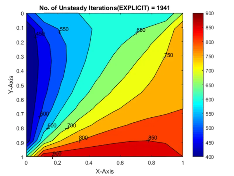
Output:
CONCLUSIONS:
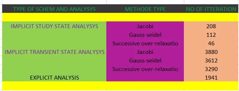
From the above outputs of various methods & comparing their No. of iterations, we can conclude that
- Jacobi > Gauss-seidel > Successive over-relaxation according to the No. of iterations computed for all methods & Schemes.
- When comparing Steady state and Unsteady state, it is proven that Steady state is the most successful one as it takes least number of iterations and least time to compute.
- SOR iteration method is the most effective iteration method as it took least No. of iterations for coverging solutions in both the schemes (EXPLICIT & IMPLICIT) compared to Jacobi & Gauss-siedel.