Week 5.1 - Mid term project - Solving the steady and unsteady 2D heat conduction problem
AIM:
Solve the 2-D heat conduction equation for steady and Transient state equation.
Given input:
The Boundary conditions for the problem are as follows;
Top Boundary = 600 K
Bottom Boundary = 900 K
Left Boundary = 400 K
Right Boundary = 800 K
implement the following methods for solving implicit equations.
- Jacobi
- Gauss-seidel
- Successive over-relaxation
Your absolute error criteria is 1e-4
2-D heat conduction equation
The 2D heat conduction equation is a partial differential equation (PDE) that describes the distribution of heat in a two-dimensional solid material over time. The equation takes the form of:
∂u/∂t = α (∂²u/∂x² + ∂²u/∂y²)
where u is the temperature at a point in the material,
t is time,
x and y are the spatial coordinates, and
α is the thermal diffusivity of the material.
This equation is used to model the heat transfer in a wide variety of engineering and physics problems.
Steady state Heat conduction
Steady state heat conduction is a type of heat transfer that occurs in a solid material when the temperature distribution within the material becomes constant with time, and the heat flow into or out of the material remains constant. In steady state heat conduction, the temperature at any point within the material does not change with time. This type of heat transfer is often used in the design of insulation systems, heat exchangers, and other applications.
`(del^2 T)/(delx^2)+(del^2 T)/(dely^2)=0`
By using iterative solvers we can solve this heat conduction equation.
Before that we assume our computational area as a square
Number of nodes in x and y directions are equal(nx=ny=10)
And also we have the given boundary conditions.
MATLAB coding
clear all
close all
clc

%Creating domain
nx=10;
ny=10;
x=linspace(0,1,nx)
y=linspace(0,1,ny)
%Temperature
T=ones(nx,ny)

%Boundary conditions
T(1,1:end)=600
T(end,1:end)=900
T(1:end,1)=400
T(:,end)=800

Told=T;%initial temperature

tol=1e-4; %Absolute error criteria
error=1;
%element size
dx=x(2)-x(1)
dy=y(2)-y(1)
k=2*(dx^2+dy^2)/(dx^2*dy^2)

omega=1.1   %Relaxation factor

iterative_solver=1;

%Jacobi method

if iterative_solver==1
    jacobi_iter=1;
    while (error>tol)
        %iteration loop
    for i=2:nx-1
        for j=2:ny-1
            %Temperature ateach grid pionts
            T(i,j)=(1/k)*(((Told((i-1),j)+Told((i+1),j))/dx^2)+((Told(i,(j-1))+Told(i,(j+1)))/dy^2));
        end
    end
    error=max(max(abs(Told-T)))
    Told=T %updating temperature
    jacobi_iter=jacobi_iter+1

    end

    %Plotting
    contour(x,y,T);
    clabel(contourf(x,y,T));
    colorbar
    colormap("jet")
    set(gca,'ydir','reverse')
    title(sprintf('No. of Iterations = %d',jacobi_iter));
end


%Gauss seidel method

if iterative_solver==2
   gs_iter=1;
    while (error>tol)
        %iteration loop
    for i=2:nx-1
        for j=2:ny-1
            %Temperature ateach grid pionts
            T(i,j)=(1/k)*(((T((i-1),j)+Told((i+1),j))/dx^2)+((T(i,(j-1))+Told(i,(j+1)))/dy^2));
        end
    end
    error=max(max(abs(Told-T)))
    Told=T %updating temperature
    gs_iter=gs_iter+1

    end

    %Plotting
    contour(x,y,T);
    clabel(contourf(x,y,T));
    colorbar
    colormap("jet")
    set(gca,'ydir','reverse')
    title(sprintf('No. of Iterations = %d',gs_iter));
end


%Successive over Relaxation method

if iterative_solver==3
   sor_iter=1;
    while (error>tol)
        %iteration loop
    for i=2:nx-1
        for j=2:ny-1
            %Temperature ateach grid pionts
            T(i,j)=Told(i,j)*(1-omega)+omega*((1/k)*(((T((i-1),j)+Told((i+1),j))/dx^2)+((T(i,(j-1))+Told(i,(j+1)))/dy^2)));
        end
    end
    error=max(max(abs(Told-T)))
    Told=T %updating temperature
    sor_iter=sor_iter+1

    end

    %Plotting
    contour(x,y,T);
    clabel(contourf(x,y,T));
    colorbar
    colormap("jet")
    set(gca,'ydir','reverse')
    title(sprintf('No. of Iterations = %d',sor_iter));
end
Output:
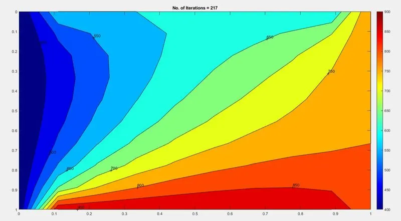
Jacobi
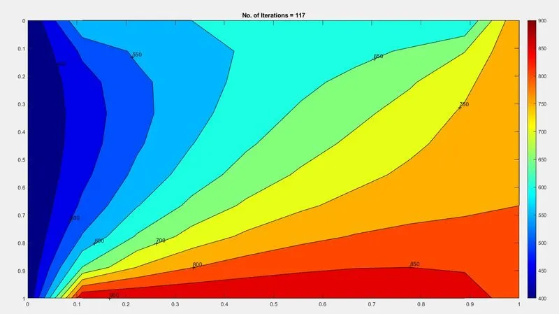
Gauss seidel
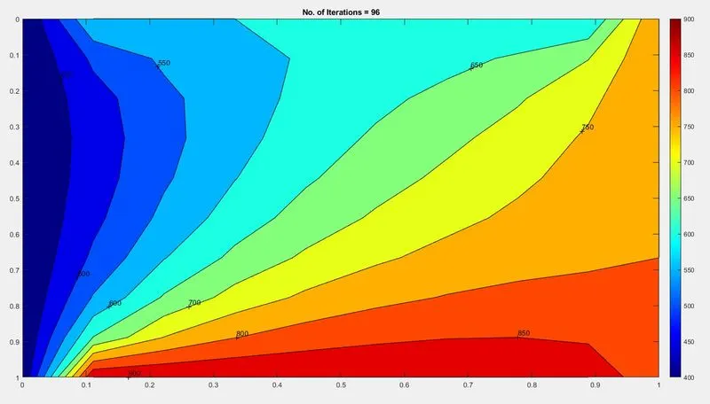
SOR
Transient state heat conduction
Transient state heat conduction is a type of heat transfer that occurs in a solid material when the temperature distribution within the material is changing with time, and the heat flow into or out of the material is also changing. In a transient state, the temperature at any point within the material is not constant and can change rapidly over time. This type of heat transfer is often used in the design of systems where the heat flow into or out of the material is not constant, such as in the heating or cooling of a building or in the manufacturing process of certain materials. The mathematical description of transient state heat conduction is based on the heat diffusion equation
the equation is given by:
∂T/∂t = α ∇²T
where T is the temperature, t is time, α is the thermal diffusivity (α = k/ρCp, where k is the thermal conductivity, ρ is the density, and Cp is the specific heat capacity), and ∇² is the Laplacian operator.
Explicit method
MATLAB Coding
clear all
close all
clc

%Creating domain
nx=10;
ny=10;
x=linspace(0,1,10)
y=linspace(0,1,10)
%defining Temperature
T=300*ones(nx,ny)

%Boundary conditions
T(1,1:end)=600
T(end,1:end)=900
T(1:end,1)=400
T(:,end)=800


Told=T;%initial temperature

tol=1e-4; %Absolute error criteria
error=1;

%element size
dx=x(2)-x(1)
dy=y(2)-y(1)
%Thermal diffusivity
alpha=1.4
dt = 1/(2*((alpha/dx^2)+(alpha/dy^2))); %time intervel


k1=(alpha*dt)/(dx)^2
k2=(alpha*dt)/(dy)^2


   iter=1;
   %convergence loop
    while (error>tol)
        %iteration loop
    for i=2:nx-1
        for j=2:ny-1
            %Temperature ateach grid pionts
            term1=Told(i-1,j)-2*Told(i,j)+Told(i+1,j)
            term2=Told(i,j-1)-2*Told(i,j)+Told(i,j+1)
            T(i,j)=Told(i,j)+k1*term1+k2*term2
        end
    end
    %maximum error for the iteration
    error=max(max(abs(Told-T)))
    Told=T %updating temperature
    %no. of iterations
    iter=iter+1


 %Plotting

    [C,H]=contourf(T);
    clabel(C,H)
    colormap("jet")
    set(gca,'ydir','reverse')
    title(sprintf('No. of Iterations = %d',iter));
    end
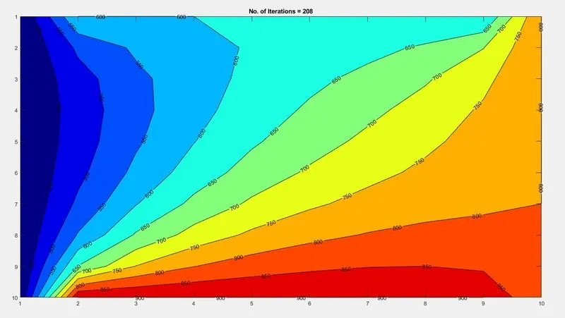
Output
Implicit method:
clear all
close all
clc

%Creating domain
nx=10;
ny=10;
x=linspace(0,1,nx)
y=linspace(0,1,ny)
%Temperature nodes
T=300*ones(nx,ny)

%Boundary conditions
T(1,1:end)=600
T(end,1:end)=900
T(1:end,1)=400
T(:,end)=800

Told=T;%initial temperature


tol=1e-4; %Absolute error criteria
error=1;
%element size
dx=x(2)-x(1)
dy=y(2)-y(1)

dt=0.01 %time intervel
nt=40 %no. of time steps
alpha=1.5  %Thermal diffusivity
omega=1.1  %Relaxation factor

k1=(alpha*dt)/(dx)^2
k2=(alpha*dt)/(dy)^2


iterative_solver=3;

%Jacobi method

if iterative_solver==1
         iter=1;
 for k=1:nt


    while (error>tol)
        %iteration loop
    for i=2:nx-1
        for j=2:ny-1


           term1=(1+2*k1+2*k2)^(-1);
            term2=k1*term1;
            term3=k2*term1;

             %Temperature at each grid pionts
            H=Told(i-1,j)+Told(i+1,j);
            V=Told(i,j-1)+Told(i,j+1);
            T(i,j)=(Told(i,j)*term1)+(H*term2)+(V*term3);
        end
    end
    error=max(max(abs(Told-T)));
    Told=T %updating temperature
    iter=iter+1

    end

    %Plotting

    [C,H]=contourf(T);
    clabel(C,H)

    colorbar
    colormap("jet")
    set(gca,'ydir','reverse')
    title(sprintf('No. of Iterations =%d',iter));
 end
 end


 %Gauss seidel method
 if iterative_solver==2
     iter=1;
 for  k=1:nt


    while (error>tol)
        %iteration loop
    for i=2:nx-1
        for j=2:ny-1

            %Temperature at each grid pionts
            term1=(1+2*k1+2*k2)^(-1);
            term2=k1*term1;
            term3=k2*term1;


            H=T(i-1,j)+Told(i+1,j);
            V=T(i,j-1)+Told(i,j+1);
            T(i,j)=(Told(i,j)*term1)+(H*term2)+(V*term3);
        end
    end
    error=max(max(abs(Told-T)));
    Told=T %updating temperature

    iter=iter+1

    end

    %Plotting

    [C,H]=contourf(T);
    clabel(C,H)

    colorbar
    colormap("jet")
    set(gca,'ydir','reverse')
    title(sprintf('No. of Iterations =%d',iter));
 end
 end


  %successive over relaxation method
 if iterative_solver==3
     iter=1;
 for  k=1:nt


    while (error>tol)
        %iteration loop
    for i=2:nx-1
        for j=2:ny-1

            %Temperature at each grid pionts

           term1=(1+2*k1+2*k2)^(-1);
            term2=k1*term1;
            term3=k2*term1;

            H=(T(i-1,j)+Told(i+1,j));
            V=(T(i,j-1)+Told(i,j+1));
            T(i,j)=Told(i,j)*(1-omega)+omega*((Told(i,j)*term1)+(H*term2)+(V*term3));
        end
    end
    error=max(max(abs(Told-T)));
    Told=T %updating temperature

    iter=iter+1

    end

    %Plotting

    [C,H]=contourf(T);
    clabel(C,H)

    colorbar
    colormap("jet")
    set(gca,'ydir','reverse')
    title(sprintf('No. of Iterations =%d',iter));
 end
end
Output:
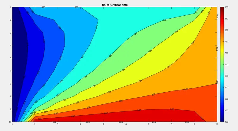
Jacobian
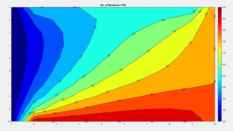
Gauss seidel method
SOR
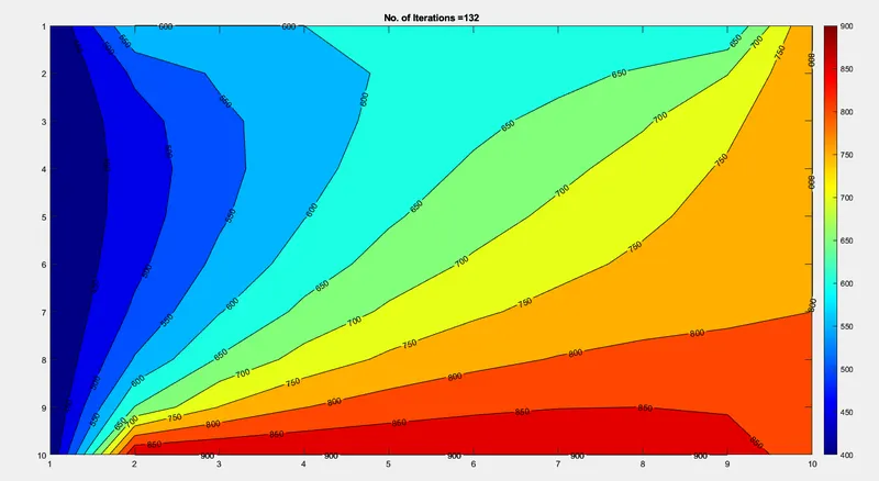
| Scheme | Iterative solver | No. of iterations |
| Steady state | Jacobi | 217 |
| Gauss seidel | 117 | |
| SOR | 96 | |
| Transient state(implicit) | Jacobi | 248 |
| Gauss seidel | 155 | |
| SOR | 132 |
Conclusion
From the above plots we can see that SOR takes minimum time for converging solutions with fewer iterations and minimum error values when compared with jacobi and gauss seidel method in seady state and Transient state.