Week 5.1 - Mid term project - Solving the steady and unsteady 2D heat conduction problem

Aim:

1. Steady state analysis & Transient State Analysis

Solve the 2D heat conduction equation by using the point iterative techniques that were taught in the class. The Boundary conditions for the problem are as follows;

Top Boundary = 600 K

Bottom Boundary = 900 K

Left Boundary = 400 K

Right Boundary = 800 K

You will implement the following methods for solving implicit equations.

• Jacobi
• Gauss-seidel
• Successive over-relaxation

Your absolute error criteria is 1e-4

Theory:

General 3-d Heat conduction equation:

`(del^2T)/(delx^2)+(del^2T)/(dely^2)+(del^2T)/(delz^2)+q/k=(1/alpha)*(delT)/(del tau)`

Code explanation:

Define the length of the domain and divide it into node points along x and y directions.

Initialize the temperature array and assign the values at the boundary as per the given criteria.

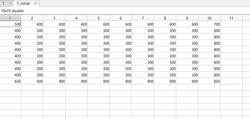
Matlab Code To solve steady state heat conduction equation:

clear all
close all
clc

% Solve 2-d steady state heat conduction euation d^2T/dx^2 + d^2T/dy^2=0


%  Inputs
l=1;              % Domain length
nx = 10;          % No of node points in x direction
ny = 10;          % No of node points in y direction

x=linspace(0,l,nx);
y=linspace(0,l,ny);

% dx = x(2) - x(1);
% dy = y(2) - y(1);

dx = l/(nx-1);

dy = l/(ny-1);

% temperature at each node point is initialized as 300 k 

T = 300 * ones(nx,ny);          

% Boundary Conditions
T(1,:)=600;
T(end,:)=900;
T(:,1)=400;
T(:,end)=800;

% Value of T at the corner nodes of boundary

T(1,1) = 500;
T(end,1) = 650;
T(1,end) = 700;
T(end,end) = 850;

% Creating a copy of T
T_old=T;

% Constants

omega=0.6;

K= ( 2 * ( dx^2 + dy^2 )) / ( dx^2 * dy^2 );

error=9e+9;

tol=1e-4;

% For jacobi method select 1, gs-2, sor-3.

iterative_solver=3;

% Jacobi Method

if iterative_solver==1
    jacobi_iter=1;

    while(error > tol)

        for i=2:nx-1

            for j=2:ny-1
    
                term1 = (T_old(i-1,j)+T_old(i+1,j))/dx^2;

                term2 = (T_old(i,j-1)+T_old(i,j+1))/dy^2;

                T(i,j) = (term1+term2)/K;

            end
        
        end
    
          error=max(abs(T_old-T));

          T_old=T;

          jacobi_iter=jacobi_iter+1;

              
    end
end

% Gauss siedel Method

if iterative_solver==2
    gs_iter=1;

    while(error > tol)

        for i=2:nx-1

            for j=2:ny-1
    
                term1 = (T(i-1,j)+T(i+1,j))/(dx^2);

                term2 = (T(i,j-1)+T(i,j+1))/(dy^2);

                T(i,j) = (term1+term2)/K;

            end

        end
       
    
        error=max(abs(T_old-T));

        T_old=T;

          gs_iter=gs_iter+1;

         
    end
end


% SOR Method

if iterative_solver==3
    sor_iter=1;

    while(error > tol)

        for i=2:nx-1

            for j=2:ny-1
    
                term1 = (T_old(i-1,j)+T_old(i+1,j))/(dx^2);

                term2 = (T_old(i,j-1)+T_old(i,j+1))/(dy^2);

               
                T(i,j)=(1-omega) * T_old(i,j) + omega * ((term1+term2)/K);

            end

        end
       
    
        error=max(abs(T_old-T));

        T_old=T;

          sor_iter=sor_iter+1;

          
    end
end

[X,Y] = meshgrid(x,y);
contourf(X,Y,T)
colorbar
set(gca,'ydir','reverse')

Matlab Code To solve unsteady state heat conduction equation:

clear all
close all
clc

% Solve 2-d steady state heat conduction euation d^2T/dx^2 + d^2T/dy^2=0


%  Inputs
l=1;              % Domain length
nx = 10;          % No of node points in x direction
ny = 10;          % No of node points in y direction
nt=1600;

x=linspace(0,l,nx);
y=linspace(0,l,ny);

% dx = x(2) - x(1);
% dy = y(2) - y(1);

dx = l/(nx-1);

dy = l/(ny-1);

% temperature at each node point is initialized as 300 k 

T = 300 * ones(nx,ny);          

% Boundary Conditions
T(1,:)=600;
T(end,:)=900;
T(:,1)=400;
T(:,end)=800;

% Value of T at the corner nodes of boundary

T(1,1) = 500;
T(end,1) = 650;
T(1,end) = 700;
T(end,end) = 850;

% Creating a copy of T
T_old=T;
T_initial=T;
T_end=T;

% Constants

dt=1e-3;

omega=1.1;

error=1e9;

tol=1e-4;

sor_iter=0;

%Calculation of 2D steady heat conduction EQUATION by Successive over-relaxation method
k1 = 1.1*(dt/(dx^2));
k2 = 1.1*(dt/(dy^2));


% Successive over relaxation Method

for k=1:nt

    while(error > tol)

        for i=2:nx-1

            for j=2:ny-1
    
                Term_1 = 1/(1 + (2*k1) + (2*k2));

                Term_2 = k1*Term_1;

                Term_3 = k2*Term_1;

                H = (T_old(i-1,j)) + (T_old(i+1,j));

                V = (T_old(i,j+1)) + (T_old(i,j-1));
                    
                T(i,j) = (T_initial(i,j)*Term_1) + (H*Term_2) + (V*Term_3);

                T_end(i,j) = ((1-omega)*T_old(i,j)) + (T(i,j)*omega);

            end
        
        end
    
          error=max(abs(T_old-T));

          T_old=T_end;

          sor_iter=sor_iter+1;

              
    end
end


[X,Y] = meshgrid(x,y);
contourf(X,Y,T)
colorbar
set(gca,'ydir','reverse')

Results and Plots:

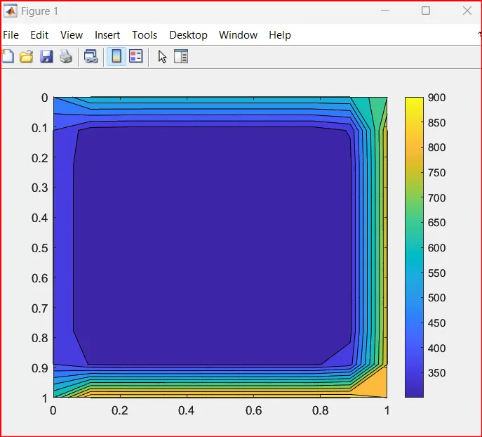
Steady state Jacobi Method

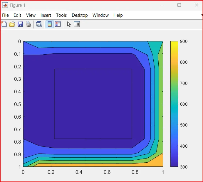
Steady state Gauss siedel Method

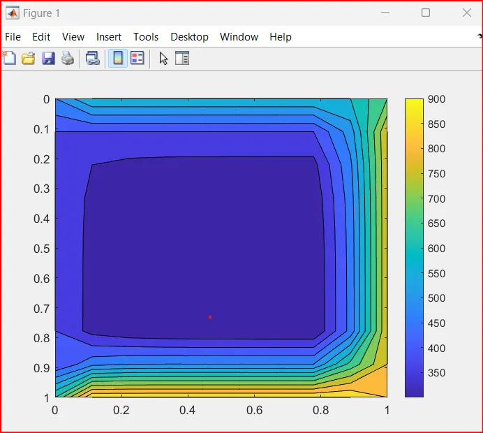
Steady state Sucessive over relaxation Method

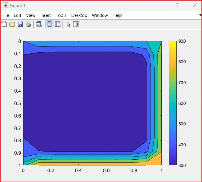
Unsteady state: