Week 11 - Simulation of Flow through a pipe in OpenFoam
In this project, I will be simulating an incompressible-laminar-axi-symmetric flow through a constant cross section for a Reynold's number of 2100. This will be solved using the software OpenFOAM running on Debian.
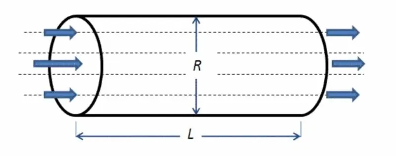
We can notice that in our case, the flow is laminar and incompressible and the solution is transient as well.
Hydrodynamic Enterance Length
It is the distance from the start of flow to the point when the flow becomes fully developed.
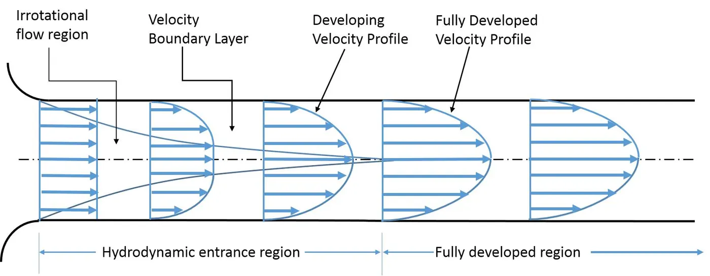
The hydrodynamic entrance region refers to the area of a pipe where fluid entering a pipe develops a velocity profile due to viscous forces propagating from the interior wall of a pipe. The flow in this region is non-uniform due to pipe friction, the length of the hydrodynamic entrance region for laminar flow is given by: L=0.06⋅Re⋅D where Re is the Reynold's Number and D is the diameter of the pipe.
For this case, Re=2100,D=0.02m. This gives a hydrodynamic entrance length of ~2.52m.
Calculation of flow
This simulation will be conducted for a Reynold's number of 2100.
Reynolds Number for a circular pipe is given by: Re=uLν where u is the inlet velocity, L is the length of the domain and ν is the kinematic viscosity.
Substituting all values and rearranging, we get: u=Re⋅νL⇒2100⋅10−50.02=1.05m/s
BlockMeshDict_generator code - This file generates a fully functional BlockMeshDict file, compiled in matlab.
Code for the generation of blockMeshDict file:
clear all
close all
clc
length = 3; % meters
radius = 0.01; % meters
theta = 4; % degrees
% input data
number_of_mesh_elements_x = 1000;
number_of_mesh_elements_y = 1;
number_of_mesh_elements_z = 10;
grading_factor_x = 1;
grading_factor_y = 1;
grading_factor_z = 1;
% opening the file
f1 = fopen("BlockMeshDict.txt",'w');
% adding comments in the file to mention input data used to generate
% BlockMeshFile
time = datestr(clock,'YYYY/mm/dd HH:MM:SS:FFF');
fprintf(f1,'FoamFilen{ntformattascii;ntclass tdictionary;ntobjecttblockMeshDict;n}');
fprintf(f1,'nn/*nFile Generated at %23s for values:nlength(m):%fnradius(m):%fntheta(deg):%d',time,length,radius,theta);
fprintf(f1,'nNumber of mesh elements in x, y, z directions respectively : (%d %d %d)nGrading Factor in x, y, z directions respectively: (%d %d %d)n*/',number_of_mesh_elements_x,number_of_mesh_elements_y,number_of_mesh_elements_z,grading_factor_x,grading_factor_y,grading_factor_z);
fprintf(f1,'nnnconvertToMeters 1;');
% starting to generate the BlockMeshDict file
fprintf(f1,'nnverticesn(');
fprintf(f1,'nt(0 0 0)');
fprintf(f1,'nt(0 %d %d)',radius*cosd(theta/2),radius*sind(theta/2));
fprintf(f1,'nt(0 %d %d)',radius*cosd(-theta/2),radius*sind(-theta/2));
fprintf(f1,'n');
fprintf(f1,'nt(%d 0 0)',length);
fprintf(f1,'nt(%d %d %d)',length,radius*cosd(theta/2),radius*sind(theta/2));
fprintf(f1,'nt(%d %d %d)',length,radius*cosd(-theta/2),radius*sind(-theta/2));
fprintf(f1,'n);');
fprintf(f1,'nnblocksn(');
fprintf(f1,'nthex (4 1 2 5 3 0 0 3) (%d %d %d) simpleGrading (%d %d %d)',number_of_mesh_elements_x,number_of_mesh_elements_y,number_of_mesh_elements_z,grading_factor_x,grading_factor_y,grading_factor_z);
fprintf(f1,'n);');
fprintf(f1,'nnedgesn(');
fprintf(f1,'ntarc 1 2 (0 %d 0)',radius);
fprintf(f1,'ntarc 4 5 (%d %d 0)',length,radius);
fprintf(f1,'n);');
fprintf(f1,'nnboundaryn(');
fprintf(f1,'ntinletnt{');
fprintf(f1,'ntttype patch;nttfacesntt(');
fprintf(f1,'nttt(0 1 2 0)');
fprintf(f1,'ntt);');
fprintf(f1,'nt}n');
fprintf(f1,'ntoutletnt{');
fprintf(f1,'ntttype patch;nttfacesntt(');
fprintf(f1,'nttt(3 5 4 3)');
fprintf(f1,'ntt);');
fprintf(f1,'nt}n');
fprintf(f1,'ntouterSurfaceWallnt{');
fprintf(f1,'ntttype wall;nttfacesntt(');
fprintf(f1,'nttt(4 5 2 1)');
fprintf(f1,'ntt);');
fprintf(f1,'nt}n');
fprintf(f1,'ntsideWallnt{');
fprintf(f1,'ntttype wedge;nttfacesntt(');
fprintf(f1,'nttt(2 5 3 0)');
fprintf(f1,'ntt);');
fprintf(f1,'nt}n');
fprintf(f1,'ntsideWall2nt{');
fprintf(f1,'ntttype wedge;nttfacesntt(');
fprintf(f1,'nttt(3 4 1 0)');
fprintf(f1,'ntt);');
fprintf(f1,'nt}n');
fprintf(f1,'ntaxis_emptynt{');
fprintf(f1,'ntttype empty;nttfacesntt(');
fprintf(f1,'nttt(0 3 3 0)');
fprintf(f1,'ntt);');
fprintf(f1,'nt}n');
fprintf(f1,'n);');
fprintf(f1,'nnmergePatchPairsn(n);');
fclose(f1);
The following commands are executed in order
icoFoam
paraFoam
This means the solution is now ready, paraFoam opens the paraView window which contains our solution.
Shear Stress plot through the diameter of the pipe:
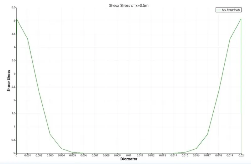
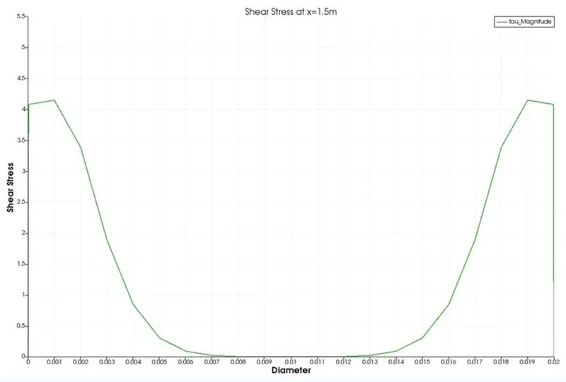
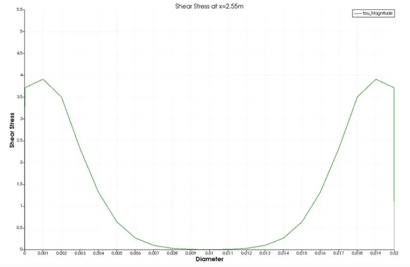
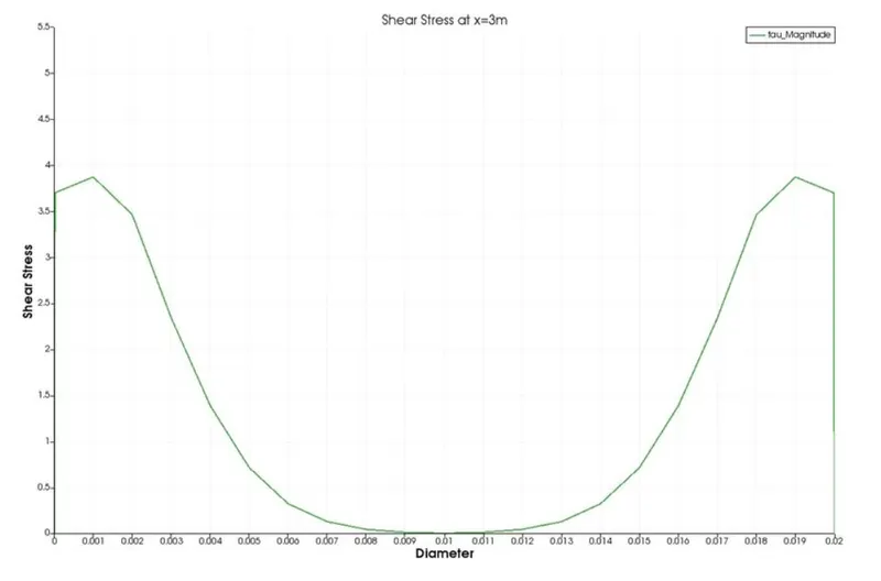
This plot shows the shear stress across the pipe's diameter. In each image, we can notice that the shear stress is maximum near the walls of the pipe due to boundary layer effect. The shear stress is maximum at the front of the pipe and gradually decreases as we approach the end of the pipe. (the y axis scale is same for all plots for easier comparison). The Shear Stress is the highest at the beginning to non-uniform flow, and is the least towards the end of the pipe as the flow becomes normal. Once fully developed flow is attained (at x~2.52m), there is no change in shear stress distribution.
Velocity plot through the diameter of the pipe:
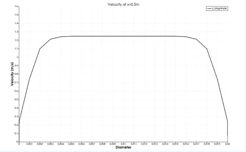
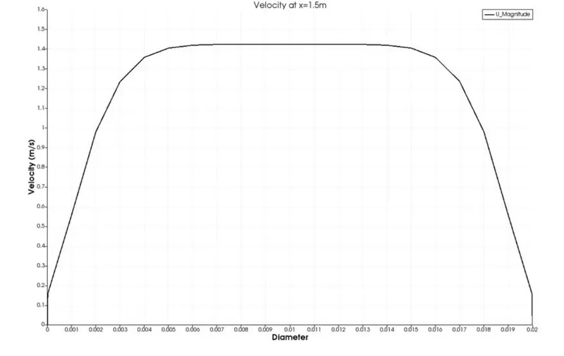
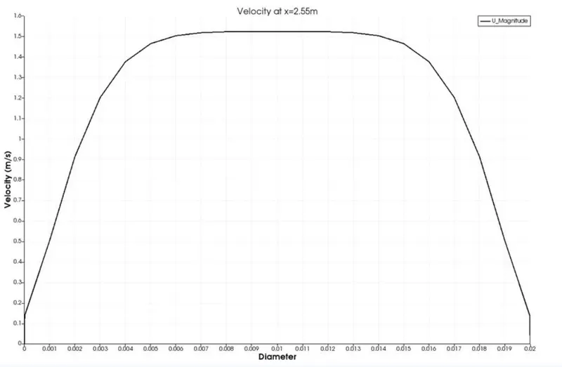
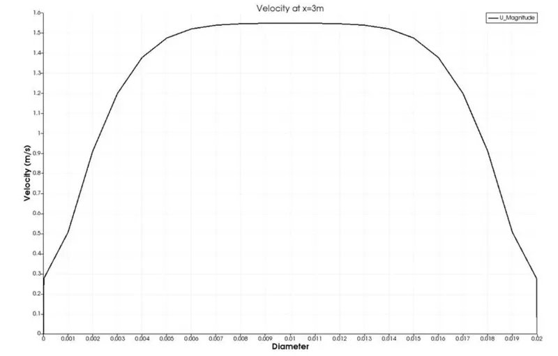
This plot shows the velocity across the pipe's diameter. In each image, we can notice that the velocity is minimum near the walls of the pipe due to boundary layer effect. The velocity increases as we approach the center of the pipe, and then. The velocity initially starts at 1 m/s and slowly moves to the fully developed velocity as the flow becomes more stable (the y axis scale is same for all plots for easier comparison). Once fully developed flow is attained (at x~2.52m), there is no major changes in velocity.
Maximum Velocity and Pressure Drop for fully developped flow
The maximum velocity Umax=Uavg⋅1.5
theoretical maximum velocity = 1.5 * 1.05 = 1.575 m/s
simulated maximum velocity = 1.548 m/s
Hagen–Poiseuille Equation/Pressure Drop for fully developed flow
The Hagen–Poiseuille equation is a physical law that gives the pressure drop in an incompressible and Newtonian fluid in laminar flow flowing through a long cylindrical pipe of constant cross section.
Δp=8μLQπR4
where Δp is the pressure drop,
μ is the dynamic viscosity,
L is the length of the pipe,
Q is the volumetric flow rate and
R is the radius of the pipe.
Substituting Q=V⋅π⋅R2,
we get Δp=8μLVR2
`substituting the values used in this simulation,
we get Δp=8⋅0.001⋅3⋅1.050.012
=252Pa
The pressure drop observed from the simulation is: 0.285 Pa (which is kinematic pressure), converting to pressure = 285 Pa.