Week 5.1 - Mid term project - Solving the steady and unsteady 2D heat conduction problem
General heat conduction equation in cartesian co-ordinate :
- [Net Heat Input] + [Heat Generated In Element] = [Change In Internal Energy]
- Final Output Equation =
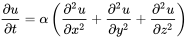
- where,
 is a real coefficient called the diffusivity of the medium.
For the 2D Equation we consider only X and Y co-ordinates. Now to solve these wuations at given boundry points we have 2 method schemes which will elaborate the heat equation
- Steady-state condition
- Unsteady/Transient state condition
To solve these equations there are iterative solvers: ERROR = [True solution] - [Approximate numerical value].
- jacobi solvers
- gauss-seidel solver
- successive over relaxation solvers
PROBLEM :
The 2D heat conduction equation by using the point iterative techniques. The following methods for solving implicit equations.
- Top Boundary = 600 K
- Bottom Boundary = 900 K
- Left Boundary = 400 K
- Right Boundary = 800 k
NOTE : w in the SOR iterations when the :
- w > 1 Over relaxation.
- w < 1 Under relaxation.
The equation for the 2D heat conduction for steady state condition :
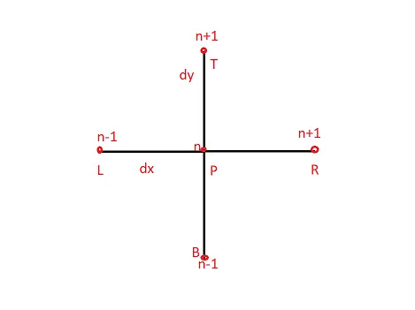
Given here is the layout for the calculation:
- [d^2T/dx^2] + [d^2T/dx^2] = 0 general form
- TP = [(1/k) (TL+TR)/ dx^2] + [(1/k) (TT+TB)/ dy^2] in discretized form
- The same equation is implimented in the matlab programme for various iterative methods mentioned above,.
The Code structure for steady solution.
clear all
close all
clc

% inputs
nx = 10; % the number of grids along x axis
ny = 10; % the number of grids along y axis
T = 300*ones(nx,ny);

% applying the boundry condition
T(1,:)= 900;
T(end,:)=600 ;
T(:,1) = 400 ;
T(:,end) = 800 ;


% add define the corner nodes
T(1,1) = 750 ;
T(nx,1) = 500 ;
T(1,ny) = 850 ;
T(nx,ny) = 700;

% creating a copy of T
Told =  T;
x = linspace(0,1,nx);
y = linspace(0,1,ny);
dx=x(2)-x(1);
dy=y(2)-y(1);
[xx,yy] = meshgrid(x,y);


% interation inputs
iterative_solver = 1;
tol = 1e-4; % tolerenace value upto how long it must solve it self to reduce its error.
error = 9e9;
k=2*((dx^2+dy^2)/(dx^2*dy^2));

%% jacobi method

if iterative_solver == 1
    jacobi_iter = 1; % we need to keep track of how many iteration we are doing
    while (error>tol)
        for i = 2:nx-1 % 2:nx-1 is the known boundry values.
            for j = 2:ny-1
                T(i,j)= (1/k)*(Told(i-1,j)+Told(i+1,j))/dx^2 +  (1/k)*(Told(i,j-1)+Told(i,j+1))/dy^2;
            end
        end
        error = max(max(abs(Told-T)));
        Told = T; % if we dont update this uold we will get the same old error from the above
        % mentioned value which is present in the input. and make
        % sure to place in this position only.
        jacobi_iter = jacobi_iter + 1 ;  % updating the va)lue just like above one.

    end
end

[c,d]=contourf(x,y,flipud(T));
colorbar
colormap(jet)
clabel(contourf(x,y,flipud(T)))
pause(0.03)
set(gca,'YDIR','reverse')
xlabel('x-axis')
ylabel('y-axis')
titletext = sprintf('iteration number = %d',jacobi_iter); % [%d] refers to iterger in
title(titletext)                                          % programming.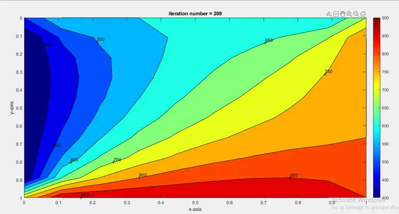
For gauss-seidel
clear all
close all
clc

% inputs
nx = 10; % the number of grids along x axis
ny = 10; % the number of grids along y axis
T = 300*ones(nx,ny);

% applying the boundry condition
T(1,:)= 900;
T(end,:)=600 ;
T(:,1) = 400 ;
T(:,end) = 800 ;

% add define the corner nodes
T(1,1) = 750 ;
T(nx,1) = 500 ;
T(1,ny) = 850 ;
T(nx,ny) = 700;

% creating a copy of T
Told =  T;
x = linspace(0,1,nx);
y = linspace(0,1,ny);
dx=x(2)-x(1);
dy=y(2)-y(1);
[xx,yy] = meshgrid(x,y);

% iteration inputs
iterative_solver = 1;
tol = 1e-4; % tolerenace value upto how long it must solve it self to reduce its error.
error = 9e9;
k=2*((dx^2+dy^2)/(dx^2*dy^2));

%% GS methods

if iterative_solver == 1
    gs_iter = 1; % we need to keep track of how many iteration we are doing
    while (error>tol)
        for i = 2:nx-1 % 2:nx-1 is the known boundry values.
            for j = 2:ny-1
                T(i,j)= (1/k)*(T(i-1,j)+Told(i+1,j))/dx^2 +  (1/k)*(T(i,j-1)+Told(i,j+1))/dy^2;
            end
        end
        error = max(max(abs(Told-T)));
        Told = T; % if we dont update this uold we will get the same old error from the above
        % mentioned value which is present in the input. and make
        % sure to place in this position only.
        gs_iter = gs_iter + 1 ;  % updating the value just like above one.

    end
end

[c,d]=contourf(x,y,flipud(T));
colorbar
colormap(jet)
clabel(contourf(x,y,flipud(T)))
set(gca,'YDIR','reverse')
pause(0.03)
xlabel('x-axis')
ylabel('y-axis')
titletext = sprintf('iteration number = %d',gs_iter); % [%d] refers to iterger in
title(titletext)                                          % programming.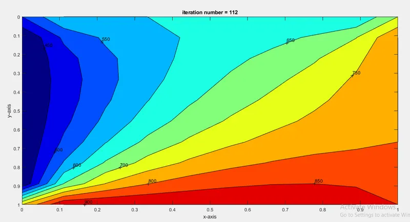
For successive over-relaxation
clear all
close all
clc

% inputs
nx = 10; % the number of grids along x axis
ny = 10; % the number of grids along y axis
T = 300*ones(nx,ny);

% applying the boundry condition
T(1,:)= 900;
T(end,:)=600 ;
T(:,1) = 400 ;
T(:,end) = 800 ;

% add define the corner nodes
T(1,1) = 750 ;
T(nx,1) = 500 ;
T(1,ny) = 850 ;
T(nx,ny) = 700;


% creating a copy of T
Told =  T;
x = linspace(0,1,nx);
y = linspace(0,1,ny);
dx=x(2)-x(1);
dy=y(2)-y(1);
[xx,yy] = meshgrid(x,y);

% interation inputs
iterative_solver = 1;
tol = 1e-4; % tolerenace value upto how long it must solve it self to reduce its error.
error = 9e9;
k=2*((dx^2+dy^2)/(dx^2*dy^2));
w = 1.1 ; % relaxation factor

%% SOR method

if iterative_solver == 1
    SOR_iter = 1; % we need to keep track of how many iteration we are doing
    while (error>tol)
        for i = 2:nx-1 % 2:nx-1 is the known boundry values.
            for j = 2:ny-1
                % T(i,j)= (1-w)*Told(i,j) + w*((1/k)*(Told(i-1,j)+Told(i+1,j))/dx^2 +  (1/k)*(Told(i,j-1)+Told(i,j+1))/dy^2);
                term1 = (T(i-1,j) + Told(i+1,j))/(dx^2);
                term2 = (Told(i,j+1) + T(i,j-1))/(dy^2);
                T(i,j) = ((Told(i,j)*(1-w))) + (w*(term1+term2))/k;
            end
        end
         error = max(max(abs(Told-T)));
    Told = T; % if we dont update this uold we will get the same old error from the above
    % mentioned value which is present in the input. and make
    % sure to place in this position only.
    SOR_iter = SOR_iter + 1 ;  % updating the value just like above one.

    end
end

[c,d]=contourf(x,y,flipud(T));
colorbar
colormap(jet)
clabel(contourf(x,y,flipud(T)))
set(gca,'YDIR','reverse')
pause(0.03)
xlabel('x-axis')
ylabel('y-axis')
titletext = sprintf('iteration number = %d',SOR_iter); % [%d] refers to iterger in
title(titletext)                                          % programming.
The equation for the 2D heat conduction for unsteady state condition/ transient state :
We are finding space derivative at (n+1)th time step
Given here is the layout for the calculation:
- ([d^2T/dx^2] + [d^2T/dx^2])*alpha = dT/dt [general form].
- TP (n+1)= term1(TP +[term2(TL+TR)^n+1]+[term3(TT+TB)^n+1]). [in discretized form].
- The same equation is implimented in the matlab programme for various iterative methods mentioned above.
The Code structure for unsteady solution.
clear all
close all
clc

% inputs
nx = 10; % the number of grids along x axis
ny = 10; % the number of grids along y axis
nt = 1400;
T = 300*ones(nx,ny);

% applying the boundry condition
T(1,:)= 900;
T(end,:)=600 ;
T(:,1) = 400 ;
T(:,end) = 800 ;


% add define the corner nodes
T(1,1) = 750 ;
T(nx,1) = 500 ;
T(1,ny) = 850 ;
T(nx,ny) = 700;

% creating a copy of T
T_prev = T;
Told =  T;
x = linspace(0,1,nx);
y = linspace(0,1,ny);
dx=x(2)-x(1);
dy=y(2)-y(1);
dt = 1e-3;
alpha = 1.2;
[xx,yy] = meshgrid(x,y);

% interation inputs
iterative_solver = 1;
tol = 1e-4; % tolerenace value upto how long it must solve it self to reduce its error.
error = 9e9;
k=2*((dx^2+dy^2)/(dx^2*dy^2));
k1 = alpha*(dt/dx^2);
k2 = alpha*(dt/dy^2);

if iterative_solver == 1 % jacobi
    jacobi_iter = 1;

    % time loop
    for nt = 1:1400
        error = 10;
        % convergence loop
        while(error>tol)
            % space loop
            for i = 2:nx-1
                for j = 2:ny-1
                    term1 = 1/(1+(2*k1)+(2*k2));
                    term2 = k1*term1;
                    term3 = k2*term1;
                    H = (Told(i-1,j)+Told(i+1,j));
                    V = (Told(i,j-1)+Told(i,j+1));
                    T(i,j)= (T_prev(i,j)*term1) + (H*term2) + (V*term3);
                end
            end

            error = max(max(abs(Told-T)));
            Told = T;
            jacobi_iter = jacobi_iter + 1 ;
        end

        T_prev=T;
    end
end

[c,d]=contourf(x,y,flipud(T));
colorbar
colormap(jet)
clabel(contourf(x,y,flipud(T)))
pause(0.03)
set(gca,'YDIR','reverse')
xlabel('x-axis')
ylabel('y-axis')
titletext = sprintf('iteration number = %d',jacobi_iter); % [%d] refers to iterger in
title(titletext)                                          % programming.
For gauss-seidel :
clear all
close all
clc

% inputs
nx = 10; % the number of grids along x axis
ny = 10; % the number of grids along y axis
nt = 1400;
alpha = 1 ;
T = 300*ones(nx,ny);

% applying the boundry condition
T(1,:)= 900;
T(end,:)=600 ;
T(:,1) = 400 ;
T(:,end) = 800 ;

% add define the corner nodes
T(1,1) = 750 ;
T(nx,1) = 500 ;
T(1,ny) = 850 ;
T(nx,ny) = 700;

% creating a copy of T
T_prev = T;
Told =  T;
x = linspace(0,1,nx);
y = linspace(0,1,ny);
dx=x(2)-x(1);
dy=y(2)-y(1);
dt = 1e-3;
[xx,yy] = meshgrid(x,y);

% interation inputs
iterative_solver = 1;
tol = 1e-4; % tolerenace value upto how long it must solve it self to reduce its error.
error = 9e9;
k=2*((dx^2+dy^2)/(dx^2*dy^2));
k1 = alpha*(dt/dx^2);
k2 = alpha*(dt/dy^2);

if iterative_solver == 1 % gauss_cidal.
    gs_iter=1;
    % time loop
    for nt = 1:1400
        error = 100 ;
        % convergence loop
        while(error>tol)
            % space loop
            for i = 2:nx-1
                for j = 2:ny-1
                    term1 = 1/(1+(2*k1)+(2*k2));
                    term2 = k1*term1;
                    term3 = k2*term1;
                    H = (T(i-1,j)) + (Told(i+1,j));
                    V = (T(i,j+1)) + (Told(i,j-1));
                    T(i,j)= (T_prev(i,j)*term1) + (H*term2) + (V*term3);
                end
            end
            error = max(max(abs(Told-T)));
            Told = T ;
            gs_iter = gs_iter + 1;
        end
        T_prev=T;
    end
end

[c,d]=contourf(x,y,flipud(T));
colorbar
colormap(jet)
clabel(contourf(x,y,flipud(T)))
pause(0.03)
set(gca,'YDIR','reverse')
xlabel('x-axis')
ylabel('y-axis')
titletext = sprintf('iteration number = %d',gs_iter); % [%d] refers to iterger in
title(titletext)                                          % programming.
clear all
close all
clc

% inputs
nx = 10; % the number of grids along x axis
ny = 10; % the number of grids along y axis
nt = 1400;
T = 300*ones(nx,ny);

% applying the boundry condition
T(1,:)= 900;
T(end,:)=600 ;
T(:,1) = 400 ;
T(:,end) = 800 ;


% add define the corner nodes
T(1,1) = 750 ;
T(nx,1) = 500 ;
T(1,ny) = 850 ;
T(nx,ny) = 700;


% creating a copy of T
T_prev = T;
Told =  T;
Tend=T;
x = linspace(0,1,nx);
y = linspace(0,1,ny);
dx=x(2)-x(1);
dy=y(2)-y(1);
dt = 1e-3;
alpha = 1;
[xx,yy] = meshgrid(x,y);

% interation inputs
iterative_solver = 1;
tol = 1e-4; % tolerenace value upto how long it must solve it self to reduce its error.
%error = 9e9;
k=2*((dx^2+dy^2)/(dx^2*dy^2));
k1 = alpha*(dt/dx^2);
k2 = alpha*(dt/dy^2);
w=1.1;

if iterative_solver == 1 % SOR
    SOR_iter=1;

    % time loop
    for nt = 1:1400
        error = 100;
        % convergence loop
        while(error>tol)
            % space loop
            for i = 2:nx-1
                for j = 2:ny-1
                    term1 = (1+(2*k1)+(2*k2))^-1;
                    term2 = k1*term1;
                    term3 = k2*term1;
                    H = (T(i-1,j)+Told(i+1,j));
                    V = (T(i,j+1)+Told(i,j-1));
                    Tgs = (term1*T_prev(i,j)) + (H*term2) + (V*term3);
                    T(i,j)= (1-w)*(Told(i,j)) + w*(Tgs);
                end
            end
            error = max(max(abs(Told-T)));
            Told = T ;
            SOR_iter = SOR_iter + 1 ;
        end
        T_prev = T;
    end
end

[c,d]=contourf(x,y,flipud(T));
colorbar
pause(0.03)
colormap(jet)
clabel(contourf(x,y,flipud(T)))
set(gca,'YDIR','reverse')
xlabel('x-axis')
ylabel('y-axis')
titletext = sprintf('iteration number = %d',SOR_iter); % [%d] refers to iterger in
title(titletext)                                          % programming.
The equation for the 2D heat conduction in EXPLICIT METHOD for Unsteady/Transient state Condition:
- ([d^2T/dx^2] + [d^2T/dx^2])*alpha = dT/dt [general form].
- TP (n+1)= TP +[k1(TL-2TP+TR)^n]+[k1(TT-2TP+TB)^n] . [in discretized form].
- The same equation is implimented in the matlab programme for various iterative methods mentioned above.
- k1 = alpha*dt/dx^2 ; k2 = alpha*dt/dy^2 ;
- k1 and k2 are the CFL numbers.
clear all
close all
clc

% inputs
nx = 10; % the number of grids along x axis
ny = 10; % the number of grids along y axis
nt = 1400;
alpha = 1.2 ;
T = 300*ones(nx,ny);

% applying the boundry condition
T(1,:)= 900;
T(end,:)=600 ;
T(:,1) = 400 ;
T(:,end) = 800 ;

% add define the corner nodes
T(1,1) = 750 ;
T(nx,1) = 500 ;
T(1,ny) = 850 ;
T(nx,ny) = 700;

% creating a copy of u
T_prev = T;
Told =  T;
x = linspace(0,1,nx);
y = linspace(0,1,ny);
dx=x(2)-x(1);
dy=y(2)-y(1);
dt = 1e-3;
[xx,yy] = meshgrid(x,y);

% interation inputs
iterative_solver = 1;
tol = 1e-4; % tolerenace value upto how long it must solve it self to reduce its error.
error = 9e9;
k=2*((dx^2+dy^2)/(dx^2*dy^2));
k1 = alpha*(dt/dx^2);
k2 = alpha*(dt/dy^2);
CFL = k1+k2

if iterative_solver == 1 % gauss_cidal.
    explicit=1;
    % time loop
    for nt = 1:1400
        error = 100 ;
        % convergence loop
       % while(error>tol)
            % space loop
            for i = 2:nx-1
                for j = 2:ny-1
                    term1 = Told(i,j);
                    term2 = k1*(Told(i+1,j) - 2*Told(i,j) + Told(i-1,j));
                    term3 = k2*(Told(i,j+1) - 2*Told(i,j) + Told(i,j-1));
                    T(i,j)= term1 + term2 + term3;
                end
            end
            error = max(max(abs(Told-T)));
            Told = T ;
            explicit = explicit + 1;
      %  end
        T_prev=T;
    end
end

[c,d]=contourf(x,y,flipud(T));
colorbar
colormap(jet)
clabel(contourf(x,y,flipud(T)))
pause(0.03)
set(gca,'YDIR','reverse')
xlabel('x-axis')
ylabel('y-axis')
titletext = sprintf('iteration number = %d',explicit); % [%d] refers to iterger in
title(titletext)                                          % programming.
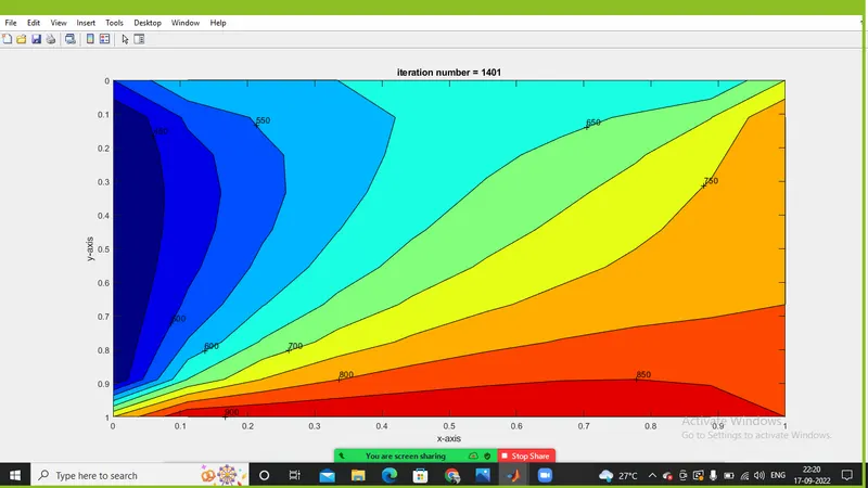
CONCLUSION AND COMPARISIONS :
For the above outputs it is clear that the iterations occuring in the implicit functions were
- JACOBI > GAUSS-SEIDEL > SOR
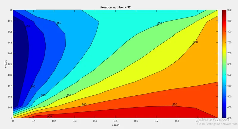
- 208 > 112 > 92 [Steady state configurations]
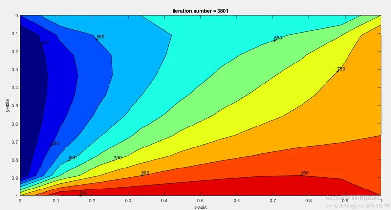
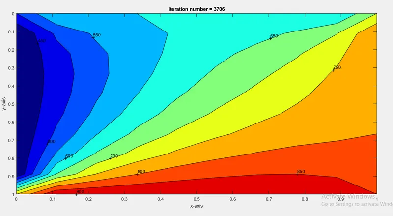
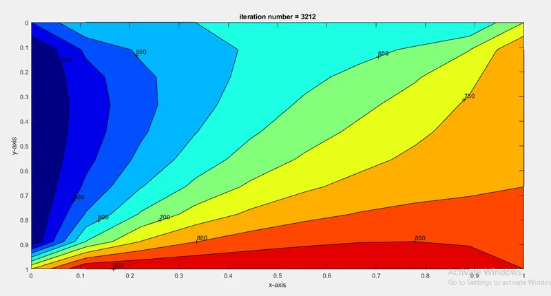
- 3801 > 3706 > 3212
For the Explicit function it is 1900.