Week 5.1 - Mid term project - Solving the steady and unsteady 2D heat conduction problem
Objective: Utilizing the following techniques, a programme can be written that solves the 2D heat conduction equation using point iterative techniques.
1. Jacobi
2. Gauss-seidel
3. Successive over-relaxation
Heat Conduction:
It is the concepts of atomic and molecular activity, for it is processes at these levels that sustain this mode of heat transfer. Conduction may be viewed as the transfer of energy from the more energetic to the less energetic particles of a substance due to interactions between the particles.
The heat flux (W/m2) is the heat transfer rate in the x direction per unit area perpendicular to the direction of transfer, and it is proportional to the temperature gradient, dT/dx, in this direction.
qx=−kdT/L;
The integrated form of the Fourier’s Law for the rate of heat conduction per unit time, Q˙, is expressed as follows:

The two terms in the aforementioned equation are term1 for the temporal derivative and term2 for the spatial derivative, where alpha is the thermal diffusivity.
Now that dimensions in the Z direction are taken into consideration under the presumption that the aforementioned equation is solved for a thin plate, the equation is transformed into the following form:
Steady-state 2D heat conduction equation:
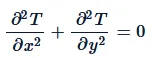
Trasient heat conduction equation:
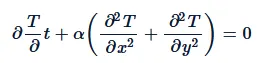
The aforementioned two equations can be resolved in two different ways utilising three iterative techniques, including Jacobi, Gauss-Seidel, and SOR.
1. Implict slover
2.explict slover
The presumption used to solve the issue is:
1. Assume that the domain is a unit square.
2. Assume nx = ny=10(for steady ) and 50 for unsteady and Doamin length=1m
3. Boundary conditions of both the cases
1. Left:400K
2. Top:600K
3. Right:800K
4. Bottom:900K
4.Tolerance=1e-4
5.Starting error=9e9
#mathcode
2D Steady-state Heat conduction:
clear all
close all
clc

%inputs for steady state problem
l=1;
nx= 20;
ny=20;
x=linspace(0,1,nx);
y=linspace(0,1,ny);
dx=l/(nx-1);
dy=l/(ny-1);
% initialising the temperature for all cells
T=300*ones(nx,ny);
Tt=600;
Tb=900;
Tr=800;
Tl=400;

%Boundary Conditions

T(:,1)=Tl;
T(:,end)=Tr;
T(1,:)=Tt;
T(end,:)=Tb;
%Edeging
T(1,1)=(Tt+Tl)*0.5;
T(1,end)=(Tr+Tt)*0.5;
T(end,1)=(Tb+Tl)*0.5;
T(end,end)=(Tb+Tr)*0.5;

T_initial=T;
Told=T;


error=9e9;

torlencevalue =1e-4;

k=2*((dx^2+dy^2)/(dx^2*dy^2)); % inputing the k value
%converging loop
%jocobi method
%Here we uses the jacobi method
Jocobi_iteration=1;

% By using the iteration solver to  determine the result of the methods
iteration_solver=input("select integer from 1,2,3\n" + ...
    "Here," + ...
    "\n1 represent Jacobi\n" + ...
    "2 represent Gauss seiden\n" + ...
    "3 represent SOR\n" + ...
    "enter integer: ");


if iteration_solver==1
    % Here while loop is been excuited given when the given values is
    % greater than the other
    while(error>torlencevalue)
        %space loop
          for i =2:(nx-1)
              for j = 2:(ny-1)

                  T(i,j)= 1/k*(((Told(i-1,j)+Told(i+1,j))/dx^2)+((Told(i,j-1)+Told(i,j+1))/dy^2));
              end
           end

         % We used to fine the maximum values
          error=max(max(abs(Told-T)));
          % here we upadating he Told values
          Told=T;
          Jocobi_iteration=Jocobi_iteration+1;


    end
    %plot
   figure(1)
   colormap(jet);
   A=contourf(x,y,T)
   clabel(A)
   set(gca,'YDir','reverse')
   xlabel('X - AXIS')
    ylabel('T')
    title(sprintf(['2 - D STEADY HEAT CONDUCTION \n Method: Jacodi \n Number of ' ...
        'Iterations : %d '], Jocobi_iteration - 1 ))
end


if iteration_solver==2;

%gauss method
%convergence value
T=T_initial;
Told=T;
error1 =9e9;
torlencevalue1=1e-4;

gauss_iteration=1;
% Here while loop is been excuited given when the given values is
    % greater than the other
while(error1>torlencevalue1)
    %space loop
    for i =2:nx-1
        for j = 2:ny-1
            T(i,j)= 1/k*(((T(i-1,j)+Told(i+1,j))/dx^2)+((T(i,j-1)+Told(i,j+1))/dy^2));
        end
    end
    gauss_iteration=gauss_iteration+1;
    %To fine the maximum values
    error1=max(max(abs(Told-T)));
    % to updated the Told
    Told=T;


end
%plot
figure(2)

    colormap(jet);
    A=contourf(x,y,T)
    clabel(A)
    set(gca,'YDir','reverse')
    title(sprintf(['2 - D STEADY HEAT CONDUCTION \n Method: Gauss seiden \n Number of ' ...
        'Iterations : %d '], gauss_iteration - 1))
end

if iteration_solver==3;
T=T_initial;
Told=T;
error3 =9e9;
torlencevalue2=1e-4;
omega =1.1;
SOR_iteration=1;
% Here while loop is been excuited given when the given values is
    % greater than the other
while (error3>torlencevalue2)
    %space loop
    for i =2:nx-1
        for j = 2:ny-1

            TSG(i,j)= 1/k*(((T(i-1,j)+Told(i+1,j))/dx^2)+((T(i,j-1)+Told(i,j+1))/dy^2));
            T(i,j)=(1-omega)*Told(i,j)+omega*TSG(i,j);
        end
    end

    SOR_iteration=SOR_iteration+1;
    %caluculating the maximum value
    error3=max(max(abs(Told-T)));
    Told=T;


end
%plot
figure(3)

    colormap(jet);
    A=contourf(x,y,T)
    clabel(A)

    set(gca,'YDir','reverse')
    title(sprintf(['2 - D STEADY HEAT CONDUCTION \n Method: SOR \n Number of ' ...
        'Iterations : %d '], SOR_iteration - 1))
end
There are two separate states: stable state and an unsteady one.
Other Schemes Include Jacobi, Gauss-Seidel, and Successive Over-Relaxation.
Various Methods to Use in an Unsteady State IMPORTANT & EXPLICIT
Use the Point Iterative Method to calculate the 2D Heat Conduction Equation, and the Jacobi, Gauss-Siedel, and SOR Iterative Methods to draw the temperature contour for stable and unsteady conditions. Additionally, use the EXPLICIT Scheme to resolve the unstable condition.
Jacobi Method:
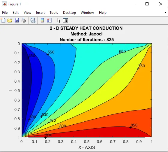
The below graph represents the Heat condctuion of the Steady using jacobi method. In that we observed that Temperature contour of the jacobi method.
The no of iteration was 825.This method assume the values are the old iteration value
Gauss seidal method:
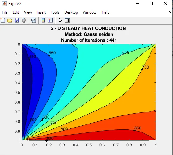
The below graph represents the Heat condctuion of the Steady using Gauss seidal method. In that we observed that Temperature contour and no of iteration required to reached it state, when compared to jacobi gauss seidal it tooks less no of iteration compare to the jacobi method. It was more effective. The reason behond is value in the gauss seiden are uptade in the same iteration.
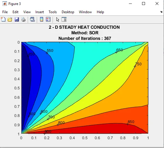
SOR:
SOR is Successive Over Relaxation. The below graph represents the Heat condctuion of the Steady using Gauss seidal method. In that we observed that Temperature contour and no of iteration required to reached it state, In SOR It can be used on jacobi and SOR Gauss seidan method, when compare to the above method it will take less iteration to compute the solution.
# Implict Unsteady analysis
%Implict function in transist function

clear all
close all
clc

%inputs for Unsteady state problem
l=1;
nx= 200;
ny=200;
x=linspace(0,1,nx);
y=linspace(0,1,ny);
dx=l/(nx-1);
dy=l/(ny-1);

% initialising the temperature for all cells
T=300*ones(nx,ny);
Tt=600;
Tb=900;
Tr=800;
Tl=400;


%Boundary Conditions

T(:,1)=Tl;
T(:,end)=Tr;
T(1,:)=Tt;
T(end,:)=Tb;
%Edeging
T(1,1)=(Tt+Tl)*0.5;
T(1,end)=(Tr+Tt)*0.5;
T(end,1)=(Tb+Tl)*0.5;
T(end,end)=(Tb+Tr)*0.5;

% inputing the values
T_initial=T;
Told=T;

% input the dt nt alpha and figures out values the values of k1 and k2
% values
dt=1e-4;
nt=800;
alpha=1.1;
k1=alpha*(dt/dx^2);
k2=alpha*(dt/dy^2);
torlence=1e-4;
Tprev=T;

% calculation of temperature distribution
Term1=1/(1+2*k1+2*k2);
Term2=k1*Term1;
Term3=k2*Term1;

iteration_solver=input("select integer from 1,2,3\n" + ...
    "Here,\n" + ...
    "1 represent Jacobi\n" + ...
    "2 represent Gauss seiden\n" + ...
    "3 represent SOR\n" + ...
    "enter integer: ")

%implict method
if iteration_solver==1
    %jacobi method
    jacobi =1;
    %time marching solution
    for k=1:nt
        error=999;
        % using the while condition for the solution
        while(error>torlence)
            %space loop
            for i = 2:nx-1
                for j= 2:ny-1
                    A = Told(i-1,j)+Told(i+1,j);
                    B=  Told(i,j+1)+Told(i,j-1);
                    T(i,j)=Term1*Tprev(i,j)+Term2*A+Term3*B;
                end
            end
            %finding the maximum values
            error=max(max(abs(Told-T)));
            %updating the values
            Told=T;
            %calculating the iterations of the solution
            jacobi = jacobi+1;
        end
        Tprev=T;

    end
    %plotting the graphs by below command
    % Fliplr command used to reverse the axis in the graph
    figure(1)
    colormap(jet);
    contourf(x,fliplr(y),T,'ShowText','on');
    pause(0.03)
    xlabel('X - AXIS')
    ylabel('T')
    title(sprintf(['2 - D UNSTEADY HEAT CONDUCTION \n Method: jacodi \n Number of ' ...
        'Iterations : %d'], jacobi - 1))
end


% if we enter integer value 2 or we have to calculate the result for the
% gauss seiden methon in implit solver then we enter the 2 in the enter the
% integer it directs to result/ graphs obtain by the gauss seiden.
if iteration_solver==2;

    %gauss seidan
    torlence1=1e-4;
    T=T_initial;
    Told=T;
    Tprev=T;
    gauss=1;
    %time marching solution
    for k=1:nt
        error1=999;
        while(error1>torlence1)
            for i = 2:nx-1
                for j= 2:ny-1
                    C=T(i-1,j)+Told(i+1,j);
                    D=T(i,j+1)+Told(i,j-1);
                    T(i,j)=Term1*Tprev(i,j)+Term2*C+Term3*D;
                end
            end
            %maximum values obtained
            error1=max(max(abs(Told-T)));
            Told=T;
            gauss = gauss+1;
        end
        Tprev=T;

    end
    %plot
    figure(2)
    colormap(jet);
    contourf(x,fliplr(y),T,'ShowText','on');
    pause(0.03)
    xlabel('X - AXIS')
    ylabel('T')
    title(sprintf(['2 - D UNSTEADY HEAT CONDUCTION \n Method: Gauss seiden \n Number of ' ...
        'Iterations : %d '], gauss - 1))

    %set(gca,'YDir','reverse')
end


% SOR method

sog=1;
if iteration_solver == 3
    omega=1.1;
    for k = 1 : nt
        error = 9e9;

        while(error > torlence)

            for i = 2:nx-1
                for j = 2:ny - 1


                    % separating the equation into two parts to avoid complexity
                    A =  (T(i-1, j) + Told(i+1, j));
                    B =  (T(i, j-1) + Told(i, j+1));
                    T(i,j) = (1 - omega) * (Told(i,j)) +(omega * ((Tprev(i,j) * Term1) + (A * Term2) + (B * Term3)));
                end
            end

            error = max(max(abs(Told-T)));
            % to update the values
            Told = T;

            sog = sog + 1;
        end
        Tprev = T;


    end
    % plot
    figure(7)
    % to flip the reversed plot
    contourf(x, fliplr(y), T, 'ShowText','on')
    pause(0.03)
    colormap(jet)
    xlabel('X - AXIS')
    ylabel('T')
    title(sprintf(['2 - D UNSTEADY HEAT CONDUCTION \n Method: SOR \n Number of ' ...
        'Iterations : %d'], sog - 1))

end
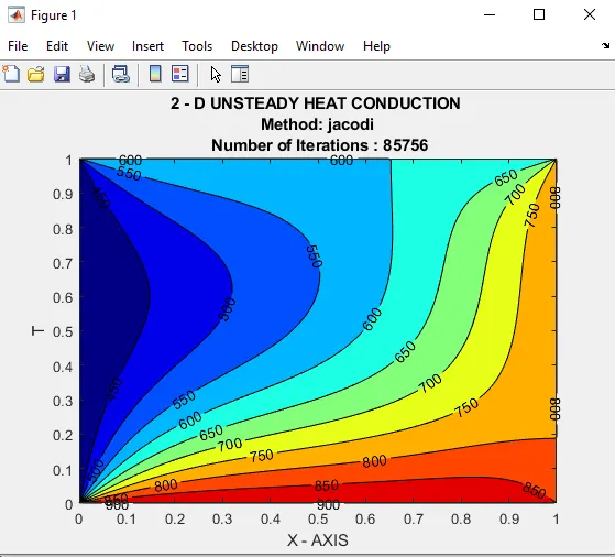
Jacobi Method:
The below graph represents the Heat condctuion of the UnSteady(implict)using jacobi method. In that we observed that Temperature contour of the jacobi method.
The no of iteration was 85756.This method assume the values are the old iteration value
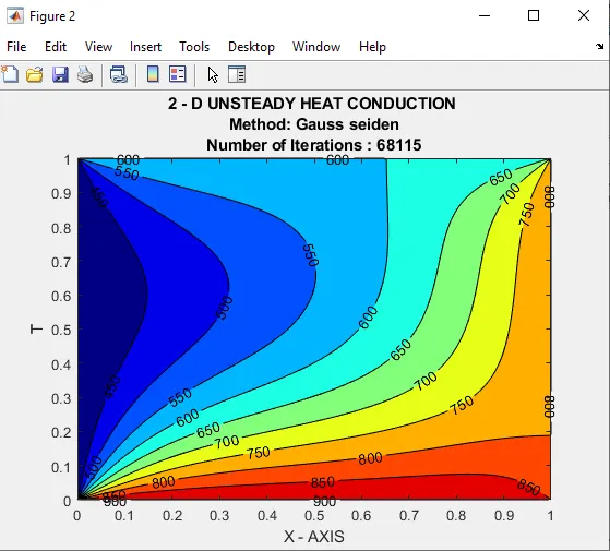
Gauss seidal method:
The below graph represents the Heat condctuion of the UnSteady(implict) using Gauss seidal method. In that we observed that Temperature contour and no of iteration required to reached it state, when compared to jacobi gauss seidal it tooks less no of iteration compare to the jacobi method. The reason behond is value in the gauss seiden are uptade in the same iteration.
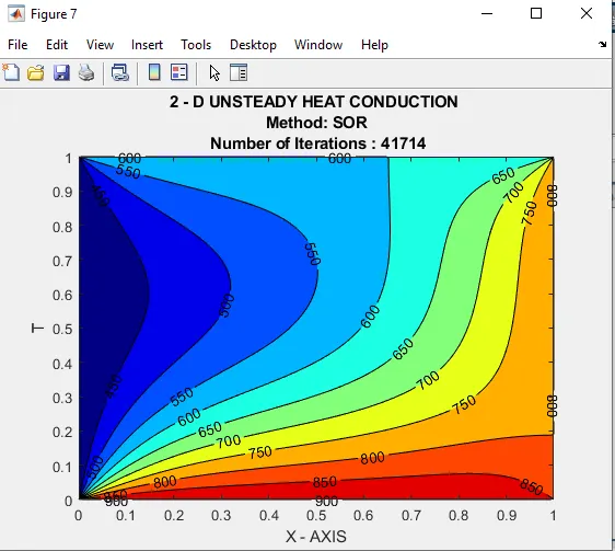
SOR:
SOR is Successive Over Relaxation. The below graph represents the Heat condctuion of the Steady using Gauss seidal method. In that we observed that Temperature contour and no of iteration required to reached it state, In SOR It can be used on jacobi and SOR Gauss seidan method, when compare to the above method it will take less iteration and time to compute the solution
#Explict Analysis
%Explict function in transist function

clear all
close all
clc

%inputs for Explict Solution
l=1;
nx= 50;
ny=50;
x=linspace(0,1,nx);
y=linspace(0,1,ny);
dx=l/(nx-1);
dy=l/(ny-1);

% initialising the temperature for all cells
T=300*ones(nx,ny);
Tt=600;
Tb=900;
Tr=800;
Tl=400;


%Boundary Conditions

T(:,1)=Tl;
T(:,end)=Tr;
T(1,:)=Tt;
T(end,:)=Tb;
%Edeging

T(1,1)=(Tt+Tl)*0.5;
T(1,end)=(Tr+Tt)*0.5;
T(end,1)=(Tb+Tl)*0.5;
T(end,end)=(Tb+Tr)*0.5;

Told=T;

dt=1;
nt=5000;
alpha=0.0001;

k1=alpha*(dt/dx^2);
k2=alpha*(dt/dy^2);
%torlence=1e-4;
cfl=k1+k2;


counter=1 ;
% time marching
for k= 1:nt
    %space loop
    for i = 2:nx-1
        for j= 2:ny-1


            A = k1*(Told(i-1,j) - 2*Told(i,j) + Told(i+1,j) );
            B = k2*(Told(i,j+1) - 2*Told(i,j) + Told(i,j-1) );
            T(i,j) = Told(i,j) + A + B;


        end
    end

    Told=T;
    counter=counter+1;

end
figure(1)

% to flip the reversed plot
contourf(x, fliplr(y), T, 'ShowText','on')
pause(0.03)
colormap(jet)
xlabel('XX')
ylabel('YY')
title(sprintf(' Method : EXPLICIT \n Iteration = %d',counter - 1));
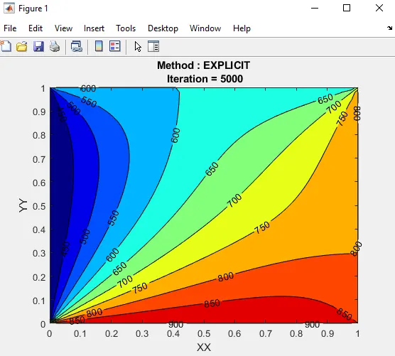
Conclusion:
| Analysis | Methods | No.of Iteration | ||||||
| Steady State (implict) |
|
|
||||||
| Un-Steady Implict Analysis |
|
|
||||||
| Un-Steady Explict Analysis | 5000 |
Jacobi is superior than Gauss-seidel and successive over-relaxation based on the calculated number of iterations for all methods and Schemes. Jacobi > Gauss-seidel > Successive over-relaxation.
Steady state is clearly more efficient than Unsteady state when compared since it takes fewer computing iterations and less time.
The SOR iteration strategy is more effective than Jacobi and Gauss-Siedel because it required less iterations to cover the solutions in both explicit and implicit schemes.