Week 5.1 - Mid term project - Solving the steady and unsteady 2D heat conduction problem

OBJECTIVE:

1. Steady state analysis & Transient State Analysis

Solve the 2D heat conduction equation by using the point iterative techniques that were taught in the class. The Boundary conditions for the problem are as follows;

Top Boundary = 600 K

Bottom Boundary = 900 K

Left Boundary = 400 K

Right Boundary = 800 K

You will implement the following methods for solving implicit equations.

1. Jacobi
2. Gauss-seidel
3. Successive over-relaxation

Your absolute error criteria are 1e-4

STEADY STATE HEAT CONDUCTION:

Under steady conditions in heat, the temperature of a body at any point does not change with time. Thus, it can be concluded that this type of heat conduction is a function of position only.

The formula for steady state heat conduction without heat generation is given by the formula:

`(del^2T)/(delx^2)+(del^2T)/(dely^2)=0`

Making use of boundary elements with the help of numerical methods. In our square domain the solutions are obtained at discrete points.

We start with the mesh and describe the profile within the domain at discrete intervals,

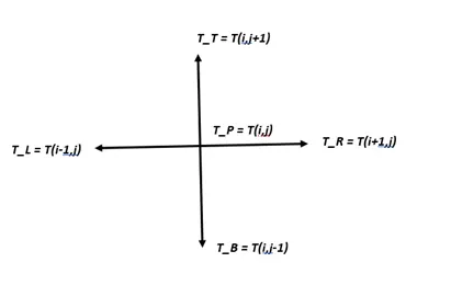
In the x & y direction the space between the two discrete points is dx and dy respectively. Now we try to formulate the problem in such a way that we can set it up as a computer program,

`(T_L-2T_P+T_R)/(delx^2)+(T_T-2T_P+T_B)/(dely^2)=0`

`(2T_P)/(delx^2)+(2T_P)/(dely^2)=[(T_L+T_R)/(delx^2)]+[(T_T+T_B)/(dely^2)]`

`T_P[(2(delx^2+dely^2))/(delx^2dely^2)]=RHS`

`K=[(2(delx^2+dely^2))/(delx^2dely^2)]`

`T_P=1/K[[(T_L+T_R)/(delx^2)]+[(T_T+T_B)/(dely^2)]]`

We assume that between any two grid points in our problem we have uniform grid spacing.

MATLAB CODE:

clear all 
close all 
clc 
 
 
%initial conditions
L=1; %length of the domain
nx=input('For the uniformly space grid please enter the number of grid points:');
ny=nx; 
 
x=linspace(0,L,nx);
y=linspace(L,0,ny);
dx=L/(nx-1); %providing the spacing between the grid points along x axis
dy=L/(ny-1); %providing the spacing between the grid points along y axis
 
error=9e9;
tol=1e-4;
 
%Defining Boundary Conditions
 
T_L=400;
T_R=800;
T_T=600;
T_B=900;
 
 
%Temperature Matrix
 
T=298*ones(nx,ny);
T(1,:)=T_B;
T(end,:)=T_T;
T(:,1)=T_L;
T(:,end)=T_R;
 
 
%Edge Refining
 
T(1,1)=(900+400)/2;
T(1,end)=(900+800)/2;
T(end,1)=(400+600)/2;
T(end,end)=(800+600)/2;
 
 
%Calculation of relaxation factor
%omega=2/(1+sin(pi*dx));
omega=1.2;
 
%Creating a copy of old values
[X,Y]=meshgrid(x,y);
Told=T;
 
 
iterative_solver=input('1) Jacobi 2) Gauss Seidel 3) SOR \nEnter an option for the type of solver you would like to use: \n');
 
k=2/dx^2 + 2/dy^2;
 
tic
if iterative_solver==1;
    jacobi_iter=1;
    while(error>tol)
        for i=2:nx-1
            for j=2:ny-1
                term1=(Told(i-1,j)+Told(i+1,j))/(k*(dx^2));
                term2=(Told(i,j-1)+Told(i,j+1))/(k*(dy^2));
                T(i,j)=term1+term2;
            end
        end
        error=max(max(abs(Told-T)));
        Told=T;
        jacobi_iter=jacobi_iter+1;
        figure(1)
        [A,B]=contourf(X,Y,T);
        set(gca,'YDIR','reverse')
        colorbar
        colormap(jet)
        clabel(A,B);
        text=sprintf('Jacobi Iterations = %d',jacobi_iter);
        ylabel('Y')
        title(text)
        pause(0.03)
    end
end
 
 
if iterative_solver==2;
    gs_iter=1;
    while(error>tol)
        for i=2:nx-1
            for j=2:ny-1
                term1=(T(i-1,j)+Told(i+1,j))/(k*(dx^2));
                term2=(T(i,j-1)+Told(i,j+1))/(k*(dy^2));
                T(i,j)=term1+term2;
            end
        end
        error=max(max(abs(Told-T)));
        Told=T;
        gs_iter=gs_iter+1;
        figure(1)
        [A,B]=contourf(X,Y,T);
        set(gca,'YDIR','reverse')
        colorbar
        colormap(jet)
        clabel(A,B);
        text=sprintf('Gauss Seidel Iterations = %d ',gs_iter);
        title(text)
        ylabel('Y')
        pause(0.03)
    end
end
 
 
if iterative_solver==3;
    sor_iter=1;
    while(error>tol)
        for i=2:nx-1
            for j=2:ny-1
                term1=(T(i-1,j)+Told(i+1,j))/(k*(dx^2));
                term2=(T(i,j-1)+Told(i,j+1))/(k*(dy^2));
                T(i,j)=(1-omega)*Told(i,j)+omega*(term1+term2);
            end
        end
        error=max(max(abs(Told-T)));
        Told=T;
        sor_iter=sor_iter+1;
        figure(1)
        [A,B]=contourf(X,Y,T);
        set(gca,'YDIR','reverse')
        colorbar
        colormap(jet)
        clabel(A,B);
        text=sprintf('SOR Iterations = %d ',sor_iter);
        title(text)
        ylabel('Y')
        pause(0.03)
    end
end
 
Time_Taken=toc

OUTPUT:

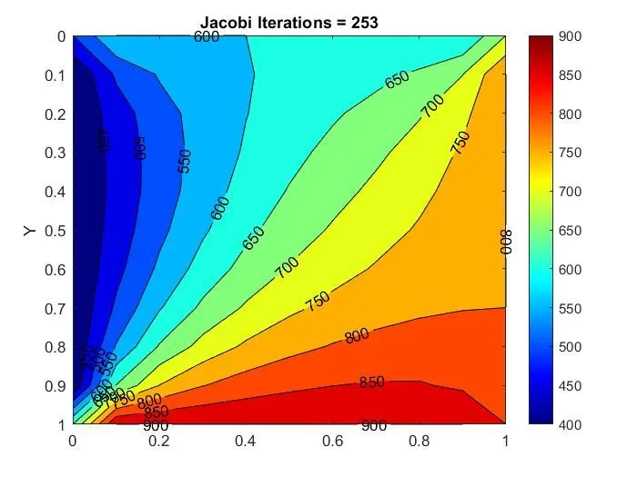
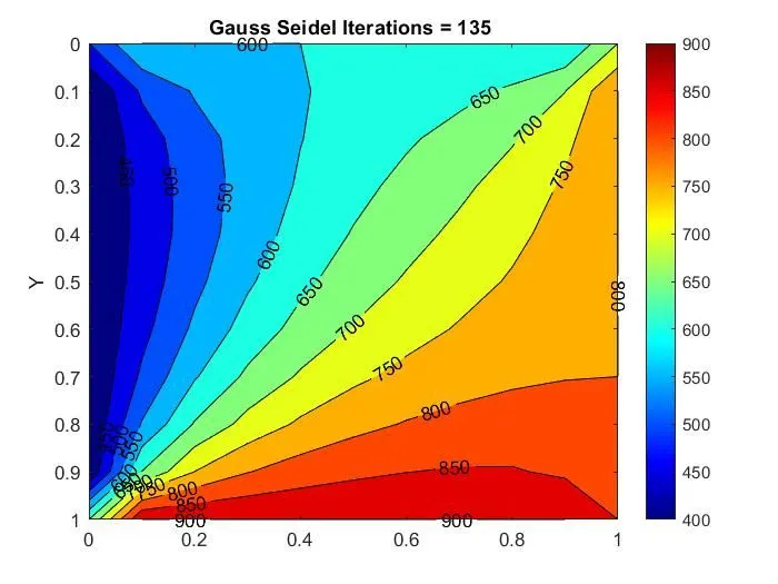
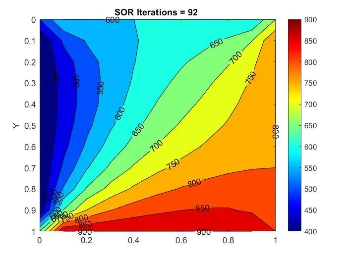
For each and every solver, we focus on Time Taken to complete the simulation and the number of iterations it takes to reach the stable solutions,

1. JACOBI:

For the uniformly space grid please enter the number of grid points:11

1) Jacobi 2) Gauss Seidel 3) SOR

Enter an option for the type of solver you would like to use: 1

Time Taken = 61.0460`

1. GAUSS SEIDEL:

For the uniformly space grid please enter the number of grid points:11

1) Jacobi 2) Gauss Seidel 3) SOR

Enter an option for the type of solver you would like to use: 2

Time Taken = 35.8623

1. SOR:

For the uniformly space grid please enter the number of grid points:11

1) Jacobi 2) Gauss Seidel 3) SOR

Enter an option for the type of solver you would like to use: 3

Time Taken = 23.5460

TRANSIENT STATE HEAT CONDUCTION:

under unsteady state conditions in heat, the temperature of a body at any point varies with time as well as position in one- dimensional and multidimensional systems. This type of heat conduction is also known as transient heat conduction. The 2D transient heat conduction equation is given by:

`(delT)/(delt)=alpha[(del^2T)/(delx^2)+(del^2T)/(dely^2)]`

In Method of Characteristics, we learned that we make use of the time marching solution when we have a time derivative in the governing equation. At each and every discrete point on the square domain this solution is implemented by making use of numerical schemes.

`(delT)/(delt)=alpha[(del^2T)/(delx^2)+(del^2T)/(dely^2)]`

`(T_P^(n+1)-T_P^n)/(delt)=alpha[(T_L-2T_P+T_R)/(delx^2)+(T_T-2T_P+T_B)/(dely^2)]^(n(or)n+1)`

`k1=alpha(delt)/(delx^2);k2=alpha(delt)/(dely^2)`

Time interval,

n is for explicit schemes

n+1 is for implicit schemes

The final equations we end up before developing it into a computer program are as follows:

For Explicit method,

`T_p^(n+1)=T_p^(n)+k1[T_L-2T_P+T_R]^n+k2[T_T-2T_P+T_B]^n`

For Implicit method,

`T_p^(n+1)=1/(1+2k1+2k2)[T_p^(n)+k1[T_L+T_R]^(n+1)+k2[T_T+T_B]^(n+1)`

EXPLICIT METHOD:

MATLAB CODE: -

clear all
close all
clc
 
 
L=1;
nx=input('For the uniformly space grid please enter the number of grid points:');
ny=nx;
 
 
x=linspace(0,L,nx);
y=linspace(L,0,ny);
dx=L/(nx-1);
dy=L/(ny-1);
 
 
dt=0.001;
%t=0.1;
%nt=t/dt;
 
 
error=9e9;
tol=1e-4;
 
 
T_L=400;
T_R=800;
T_T=600;
T_B=900;
 
 
T=298*ones(nx,ny);
T(1,:)=T_B;
T(end,:)=T_T;
T(:,1)=T_L;
T(:,end)=T_R;
 
 
T(1,1)=(900+400)/2;
T(1,end)=(900+800)/2;
T(end,1)=(400+600)/2;
T(end,end)=(800+600)/2;
 
 
alpha=1.4; %Diffusivity 
k1=alpha*dt/dx^2;
k2=alpha*dt/dy^2;
 
 
[X,Y]=meshgrid(x,y);
Told=T;
 
 
CFL=k1+k2 %To verify if the solution is stable within the limit CFL(x)+CFL(y)=0.5
unsteady_explicit_iter=1;
 
 
tic
for nt=1:1400
    while(error>tol)
        for i=2:nx-1
            for j=2:ny-1
                term1=Told(i-1,j)-2*Told(i,j)+Told(i+1,j);
                term2=Told(i,j-1)-2*Told(i,j)+Told(i,j+1);
                T(i,j)=Told(i,j)+k1*term1+k2*term2;
            end
        end
        error=max(max(abs(Told-T)));
        Told=T;
        unsteady_explicit_iter=unsteady_explicit_iter+1;
        
        
        figure(1)
        [A,B]=contourf(X,Y,T);
        set(gca,'YDIR','reverse')
        colorbar
        colormap(jet)
        clabel(A,B);
        text=sprintf('Unsteady Explicit Iterations = %d',unsteady_explicit_iter);
        ylabel('Y')
        title(text)
        pause(0.03)
    end
end
 
Time_Taken=toc

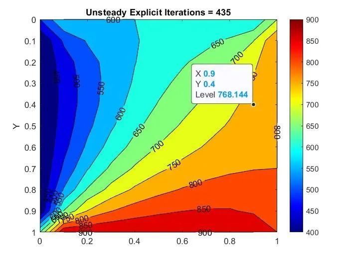
OUTPUT:

For each and every solver, we focus on Time Taken to complete the simulation and the number of iterations it takes to reach the stable solutions and CFL,

For the uniformly space grid please enter the number of grid points:11

CFL =0.2800

Time Taken =78.4365

IMPLICIT METHOD:

MATLAB CODE: -

clear all
close all
clc
 
 
L=1;
nx=input('For the uniformly space grid please enter the number of grid points:');
ny=nx;
 
x=linspace(0,L,nx);
y=linspace(L,0,ny);
 
dx=1/(nx-1);
dy=1/(ny-1);
 
alpha=1.4;
dt=0.001;
 
%error=9e9
tol=1e-4;
 
T_L=400;
T_R=800;
T_T=600;
T_B=900;
 
T=298*ones(nx,ny);
T(1,:)=T_B;
T(end,:)=T_T;
T(:,1)=T_L;
T(:,end)=T_R;
 
T(1,1)=(900+400)/2;
T(1,end)=(900+800)/2;
T(end,1)=(400+600)/2;
T(end,end)=(800+600)/2;
 
k1=alpha*dt/dx^2;
k2=alpha*dt/dy^2;
 
CFL=k1+k2
 
Told=T;
T_prev_dt=T;
iter=1;
 
omega=1.1;
 
iterative_solver=input('1) Jacobi 2) Gauss Seidel 3) SOR \nEnter an option for the type of solver you would like to use: \n');
 
tic
for nt=1:1400
    if iterative_solver==1
        
        term1=(1+2*k1+2*k2)^(-1);
        term2=k1*term1;
        term3=k2*term1;
        
        error=9e9;
        while(error>tol)
            for i=2:nx-1
                for j=2:ny-1
                    
                    H=(Told(i-1,j)+Told(i+1,j));
                    V=(Told(i,j-1)+Told(i,j+1));
                    T(i,j) = (T_prev_dt(i,j)*term1)+(H*term2)+(V*term3);
                end
            end
            
            error=max(max(abs(Told-T)));
            Told=T;
            iter=iter+1;
        end
    end
    
    if iterative_solver==2
        
        term1=(1+2*k1+2*k2)^(-1);
        term2=k1*term1;
        term3=k2*term1;
        
        error=9e9;
        while(error>tol)
            for i=2:nx-1
                for j=2:ny-1
                    
                    H=(T(i-1,j)+Told(i+1,j));
                    V=(T(i,j-1)+Told(i,j+1));
                    T(i,j) = (T_prev_dt(i,j)*term1)+(H*term2)+(V*term3);
                end
            end
            
            error=max(max(abs(Told-T)));
            Told=T;
            iter=iter+1;
        end
    end
    
    if iterative_solver==3
        
        term1=(1+2*k1+2*k2)^(-1);
        term2=k1*term1;
        term3=k2*term1;
        
        error=9e9;
        while(error>tol)
            for i=2:nx-1
                for j=2:ny-1
                    
                    H=(T(i-1,j)+Told(i+1,j));
                    V=(T(i,j-1)+Told(i,j+1));
                    T(i,j) = (1-omega)*Told(i,j)+omega*((T_prev_dt(i,j)*term1)+(H*term2)+(V*term3));
                end
            end
            
            error=max(max(abs(Told-T)));
            Told=T;
            iter=iter+1;
        end
    end
    T_prev_dt=T;
end
Time_Taken=toc
 
 
figure(1)
[P Q]=contourf(x,y,T);
set(gca,'YDIR','reverse')
colorbar;
colormap(jet);
clabel(P,Q);
text=sprintf('Implicit Iterations = %d',iter);
ylabel('Y')
title(text)
%pause(0.03)

OUTPUT:

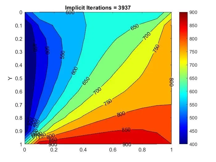
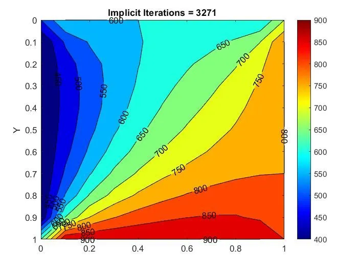
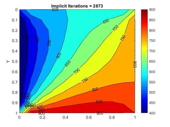
For each and every solver, we focus on Time Taken to complete the simulation and the number of iterations it takes to reach the stable solutions and CFL,

1. JACOBI METHOD:

For the uniformly space grid please enter the number of grid points:11

CFL = 0.2800

1) Jacobi 2) Gauss Seidel 3) SOR

Enter an option for the type of solver you would like to use: 1

Time Taken = 0.0944

1. GAUSS SEIDEL METHOD:

For the uniformly space grid please enter the number of grid points:11

CFL = 0.2800

1) Jacobi 2) Gauss Seidel 3) SOR

Enter an option for the type of solver you would like to use: 2

Time Taken = 0.0589

1. SOR:

For the uniformly space grid please enter the number of grid points:11

CFL = 0.2800

1) Jacobi 2) Gauss Seidel 3) SOR

Enter an option for the type of solver you would like to use: 3

Time Taken = 0.0670

RESULTS AND DISCUSSIONS:

• There is no time loop and the results converge within a few iterations, in steady state methods,. We include time loop for implicit methods and it runs for a large number of iterations.
• As it is a function of both time and position Transient solvers take a lot of time for computation, when comparing to steady state solver which is only a function of position.
• The SOR provides us the answer with a smaller number of iterations and takes less computation time.

CONCLUSION:

• The 2D heat conduction equation was solved making use of iterative techniques.