Week 5.1 - Mid term project - Solving the steady and unsteady 2D heat conduction problem
AIM
To solve the steady and unsteady 2D heat conduction problem
Equation:
`((del T)/(del t) - (alpha)((del^2 T)/(del x^2)+(del^2 T)/(del y^2)) = 0`
In physics and mathematics the heat equation is a partial differential equation that describes how the distribution of some quantity (such as heat) evolves over time in a solid medium, as it spontaneously flows from places where it is higher towards places where it is lower. It is a special case of the diffusion equation.
Given,
I have generated a 2D profile of temperature which gets analyzed. The temperature at 4 boundaries are given as below
Top=400K
Bottom=900k
Left=600K
Right=800K
1) Jacobian Iterative Solver :
In jacobi method , each iteration is done using a set of previous values, even if new values are available in the middle of an iteration.Like when you are solving for n+1 iteration and for i th node you will use values of previous(n) iteration even if you have the updated values of the nodes in current iteration.so this method is called method of simultaneous displacements.
The 2D steady state heat conduction equation for this method is
Gauss-Seidel iterative solver :
In Gauss-Seidel, as soon as you find a new value in the current iteration you will use it for finding other values in the current iteration.
Like when you are solving for n+1 iteration and for i th node you will use all the available values upto i-1 node of current iteration(n+1) and use i+1 node values and above values of previous iteration(n).SO we get more converged values.so this method is called method of spontaneous displacements.
The 2D steady state heat conduction equation for this method is
Successive Over-Relaxation( SOR) method :
It is a variant of the Gauss-Seidel method for solving a linear system of equations, resulting in faster convergence.You can also use jacobi method .Here an extra term called relaxation factor (omega)is multiplied to gauss seidel generated term to scale the convergence rate and solve the equation faster.To calculate new value we take old value and take a parameter omega and take rate of change.
The 2D steady state heat conduction equation for this method is
for scaling jacobian method,where Tj is the result of jacobian method.
and for scaling Gauss-Seidel method,where Tj is the result of Gauss-Seidel method.
when omega = 0 we get new value is equal to old value which gives wrong result.
when omega goes from 0 to 1 we are switching from no update to an update using gauss siedal or jacobi method.
when omega >1 then we are taking the update from gauss siedal method and scaling up the convergence rate. The value we give is called over relaxition factor.
when omega <1 ,The value we give is called under relaxition factor.This is used when the solution given by gauss siedel is over relaxed we give omega value less than 1 to get the converged solution.
Input Variable:
- Nodes: we are going to take no. of nodes in X-direction,nx and in Y-direction,ny=20
- Length of the domain: This is taken as 1 along x-axis and y-axis.
- Given, Tolerance assumed to be 1e-4.
- And we also assumed error as 999 .we can assume any value but it must be greater than the required tolerance.
By taking these as inputs we create a function for each solver and use those function in the main program and solve the 2D steady state equation on a square domain.
Program:
% Solving the steady state 2D heat conduction problem using iterative solvers over a square domain.
clear
close all
clc
%intial Conditions
L=1;
nx=20;
ny=nx;
tol=1e-4;
% TEMPERATURE matrix

error=9e9;
solver_number = input('enter_the_solver_number: ')

if solver_number==1
%function for steady_state_jacobian_iteration_method
steady_state_jacobian_itteration(L,nx,ny,error,tol)
end

if solver_number ==2
    %function for stady sate guass seidal iteration method
    steady_state_gauss_itteration(L,nx,ny,error,tol)
end
if solver_number ==3
    %function for stady sate SOR method
   stead_state_SOR_itteration(L,nx,ny,error,tol)
endfunction steady_state_jacobian_itteration(L,nx,ny,error, tol)
tic
x = linspace(0,L,nx);
y = linspace(0,L,ny);
dx = L/(nx-1);
dy = L/(ny-1);
% temperrature inside the grid
T = 350*ones(nx ,ny);
%boundary conditions sides
T_L = 400;
T_R = 800;
T_T = 600;
T_B = 900;
T(:,1)=T_L;
T(:,end)=T_R;
T(1,:)=T_T;
T(end,:)=T_B;
%corner point temperatures
T(1,1) = (T_L+T_T)/2;
T(1,end) = (T_T+T_R)/2;
T(end,1) = (T_L+T_B)/2;
T(end,end) = (T_B+T_R)/2;
k=(2*(dx^2+dy^2))/(dx^2*dy^2);
TOld = T;
jcob_iter_num = 1;
% Convergence loop
while error > tol
%nodal loop
for i = 2:(nx-1)
for j=2:(ny-1)
T(i,j)=(1/k)*((TOld(i-1,j)+TOld(i+1,j))/dx^2 + (TOld(i,j-1)+TOld(i,j+1))/(dy^2));
end
end
error = max(max(abs(TOld-T)));
TOld = T;
jcob_iter_num = jcob_iter_num + 1;
figure(1)
[C,h]=contourf(x,fliplr(y),T);
clabel(C,h);
colormap(jet)
colorbar;
time_required = toc
title("Jcob iteration method")
xlabel('X Axis')
ylabel('Y Axis')
end
endfunction steady_state_gauss_itteration(L,nx,ny,error,tol)
tic
x = linspace(0,L,nx);
y = linspace(0,L,ny);
dx = L/(nx-1);
dy = L/(ny-1);
% temperrature inside the grid
T = 10*ones(nx ,ny);
%boundary conditions sides
T_L = 400;
T_R = 800;
T_T = 600;
T_B = 900;
T(:,1)=T_L;
T(:,end)=T_R;
T(1,:)=T_T;
T(end,:)=T_B;
%corner point temperatures
T(1,1) = (T_L+T_T)/2;
T(1,end) = (T_T+T_R)/2;
T(end,1) = (T_L+T_B)/2;
T(end,end) = (T_B+T_R)/2;
k=(2*(dx^2+dy^2))/(dx^2*dy^2);
TOld = T;
gauss_iter_num = 1;
% Convergence loop
while error > tol
%nodal loop
for i = 2:(nx-1)
for j=2:(ny-1)
T(i,j)=(1/k)*((T(i-1,j)+TOld(i+1,j))/dx^2 + (T(i,j-1)+TOld(i,j+1))/(dy^2));
end
end
error =max(max(max(abs(TOld-T))));
TOld = T;
gauss_iter_num = gauss_iter_num + 1;
figure(1)
[C,h]=contourf(x,fliplr(y),T);
clabel(C,h);
colormap(jet)
colorbar;
time_required = toc
title("gauss seider iteration method")
xlabel('X Axis')
ylabel('Y Axis')
end
endfunction stead_state_SOR_itteration(L,nx,ny,error,tol)
tic
x = linspace(0,L,nx);
y = linspace(0,L,ny);
dx = L/(nx-1);
dy = L/(ny-1);
% temperrature inside the grid
T = 10*ones(nx ,ny);
%boundary conditions sides
T_L = 400;
T_R = 800;
T_T = 600;
T_B = 900;
T(:,1)=T_L;
T(:,end)=T_R;
T(1,:)=T_T;
T(end,:)=T_B;
%corner point temperatures
T(1,1) = (T_L+T_T)/2;
T(1,end) = (T_T+T_R)/2;
T(end,1) = (T_L+T_B)/2;
T(end,end) = (T_B+T_R)/2;
k=(2*(dx^2+dy^2))/(dx^2*dy^2);
TOld = T;
omega = 1.1;
sor_iter_num = 1;
% Convergence loop
while error > tol
%nodal loop
for i = 2:(nx-1)
for j=2:(ny-1)
Tgs(i,j)=(1/k)*((T(i-1,j)+TOld(i+1,j))/dx^2 + (T(i,j-1)+TOld(i,j+1))/(dy^2));
T(i,j)=(1-omega)*(TOld(i,j))+omega*(Tgs(i,j));
end
end
error =max(max(abs(TOld-T)));
TOld = T;
sor_iter_num = sor_iter_num + 1;
figure(1)
[C,h]=contourf(x,fliplr(y),T);
clabel(C,h);
colormap(jet)
colorbar;
time_required = toc
title("SOR method")
xlabel('X Axis')
ylabel('Y Axis')
end
endResult for steady state
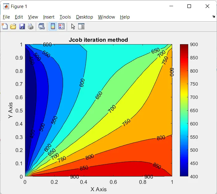
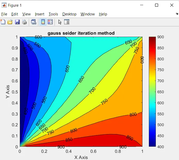
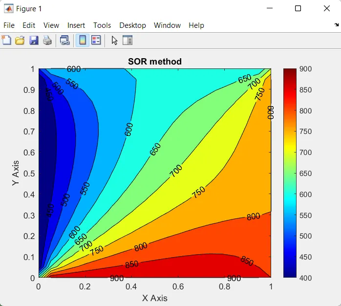
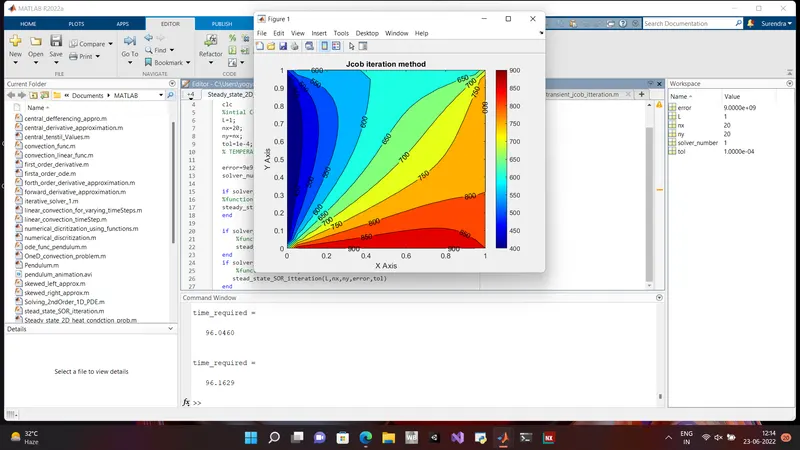
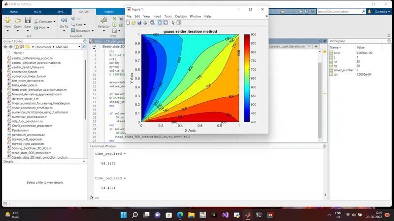
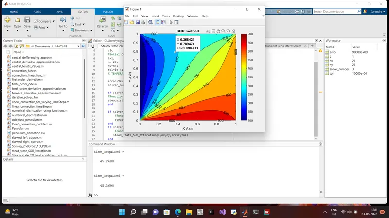
In the above three plot results you can see that the number of iterations and the computation time for jacobi iteration method is high i.e,826 iterations and 189.158 seconds time and then it is for gauss seidel method with 442 iterations and 101.2 seconds time and then for SOR.On addition of over relaxation factor to the gauss seidel method i.e, SOR method you can see that the solution is calculated in just 59 iterations and 14.3 seconds time.The SOR method depends on relaxation factor and the solution is optimum with less number of iterations and computational time when the omega value is 1.72 and the value above or below this the number iterations gets increased and when the value is above 1.99 the solution is getting blow up.so the maximum value of omega must be less than 2.you can see the blown up result if it is given greater than 2 in the below image.
Solving 2D heat conduction equation of transient state :
The equation for 2D heat conduction equation of transient state is
where alpha is the thermal diffusivity.
Then discretize the equation by using forward difference scheme for time and central difference for space.
Here we have a classification,
1) If we consider RHS terms of n th time step while calculating for (n+1) time step then we call it as explicit form.
and simplifying the equation further we get,
As it is of explict form it easy to solve these equations as we use previous time step values which are already known . we solve these equations directly by keeping it in the time loop and space loop.
Program for transient method
% Solving the steady state 2D heat conduction problem using iterative solvers over a square domain.
clear
close all
clc
%intial Conditions
L=1;
nx=20;
ny=nx;
tol=1e-4;
% TEMPERATURE matrix

error=9e9;
solver_number = input('enter_the_solver_number: ')

if solver_number==1
    %function for transient jacobian iteration_method
    transient_jcob_itteration(L,nx,ny,error,tol)
end

if solver_number ==2
    %function for transient guass seidal iteration method
    transient_gauss_itteration(L,nx,ny,error,tol)
end
if solver_number ==3
    %function for transient SOR method
   transient_SOR_itteration(L,nx,ny,error,tol)
end
Functions
function transient_jcob_itteration(L,nx,ny,error,tol)
tic
x = linspace(0,L,nx);
y = linspace(0,L,ny);
%meshing
dx = L/(nx-1);
dy = L/(ny-1);

% temperrature inside the grid
T = 300*ones(nx ,ny);

T_L = 400;
T_R = 800;
T_T = 600;
T_B = 900;
%boundary conditions
T(:,1)=T_L;
T(:,end)=T_R;
T(1,:)=T_T;
T(end,:)=T_B;
%corner point temperatures
T(1,1) = (T_L+T_T)/2;
T(1,end) = (T_T+T_R)/2;
T(end,1) = (T_L+T_B)/2;
T(end,end) = (T_B+T_R)/2;
%initial condtions
Tprev=T;
TOld = T;
dt=1e-4;
t=0.15;
nt=t/dt;
alpha=1;
k1=alpha*(dt/dx^2);
k2=alpha*(dt/dy^2);

%counter
jcob_iter_num = 1;
%time loop
for k = 1:nt
    error = 999;

% Convergence loop
    while error > tol
        %nodal loop
        for i = 2:(nx-1)
            for j=2:(ny-1)
                T(i,j)=(Tprev(i,j)+k1*(TOld(i-1,j)+TOld(i+1,j)) + k2 *(TOld(i,j-1)+TOld(i,j+1)))/(1+(2*k1)+(2*k2));
            end
        end
        error =max(max(max(abs(TOld-T))));
        TOld = T;
        jcob_iter_num = jcob_iter_num + 1;
    end
    Tprev = T;
    figure(1)
    [C,h]=contourf(x,fliplr(y),T);
    clabel(C,h);
    colormap(jet)
    colorbar;
    time_required = toc
    title("transient jcob iteration method")
    xlabel('X Axis')
    ylabel('Y Axis')
end
end
function transient_gauss_itteration(L,nx,ny,error,tol)
tic
x = linspace(0,L,nx);
y = linspace(0,L,ny);
dx = L/(nx-1);
dy = L/(ny-1);
% temperrature inside the grid
T = 300*ones(nx, ny);
%boundary conditions sides
T_L = 400;
T_R = 800;
T_T = 600;
T_B = 900;
%boundary conditions
T(:,1)=T_L;
T(:,end)=T_R;
T(1,:)=T_T;
T(end,:)=T_B;
%corner point temperatures
T(1,1) = (T_L+T_T)/2;
T(1,end) = (T_T+T_R)/2;
T(end,1) = (T_L+T_B)/2;
T(end,end) = (T_B+T_R)/2;
% initial conditions
Tprev=T;
TOld = T;
dt=1e-4;
t=0.15;
nt=t/dt;
alpha=1;
k1=alpha*(dt/dx^2);
k2=alpha*(dt/dy^2);
%counter
gauss_iter_num = 1;
%time loop
for k = 1:nt
error = 999;
% Convergence loop
while error > tol
%nodal loop
for i = 2:(nx-1)
for j=2:(ny-1)
T(i,j)=(Tprev(i,j) + k1*(T(i-1,j)+TOld(i+1,j)) + k2*(T(i,j-1) + TOld(i,j+1)))/(1+(2*k1)+(2*k2));
end
end
error =max(max(abs(TOld-T)));
%updation of TOld
TOld = T;
gauss_iter_num = gauss_iter_num + 1;
end
%updation of Tprev
Tprev = T;
%contour plotting
figure(1)
[C,h]=contourf(x,fliplr(y),T);
clabel(C,h);
colormap(jet)
colorbar;
time_required = toc
title("transient gauss seider iteration method")
xlabel('X Axis')
ylabel('Y Axis')
end
end% Function to solve 2D transient state heat conduction equation using SOR solver
function transient_SOR_itteration(L,nx,ny,error,tol)
tic
x=linspace(0,L,nx);
y=linspace(0,L,ny);
dx=L/(nx-1);
dy=L/(ny-1);
% TEMPERATURE matrix
T= 300*ones(nx,ny);
T_L = 400;
T_R = 800;
T_T = 600;
T_B = 900;
%Boundary conditions
T(:,1)=T_L;
T(:,end)=T_R;
T(1,:)=T_T;
T(end,:)=T_B;
%corner temperatures
T(1,1) = (T_L+T_T)/2;
T(1,end) = (T_T+T_R)/2;
T(end,1) = (T_L+T_B)/2;
T(end,end) = (T_B+T_R)/2;
%initial conditions
Tprev=T;
TOld =T;
dt=1e-4;
t=0.15;
nt=t/dt;
alpha=1;
% Tgs=ones(nx,ny)
k1=alpha*(dt/dx^2);
k2=alpha*(dt/dy^2);
SOR_iteration_number=1
omega=1.2;
%time loop
for k=1:nt
error =999;
% convergence loop
while(error>tol)
%nodal loop
for i=2:nx-1
for j=2:ny-1
Tgs(i,j)=(Tprev(i,j)+k1*(T(i-1,j)+TOld(i+1,j))+k2*(T(i,j-1)+TOld(i,j+1)))/(1+2*k1+2*k2);
T(i,j)=(1-omega)*TOld(i,j)+omega*Tgs(i,j);
end
end
error=max(max(abs(T-TOld)));
%updation of TOLd
TOld=T;
SOR_iteration_number= SOR_iteration_number+1;
end
%updation of previou T
Tprev=T;
figure(1)
% countour Plotting
[C,h]=contourf(x,fliplr(y),T);
clabel(C,h);
colormap(jet)
colorbar;
time_required=toc
title('transient SOR method');
xlabel('X axis')
ylabel('Y axis')
end
endResult for transient methods
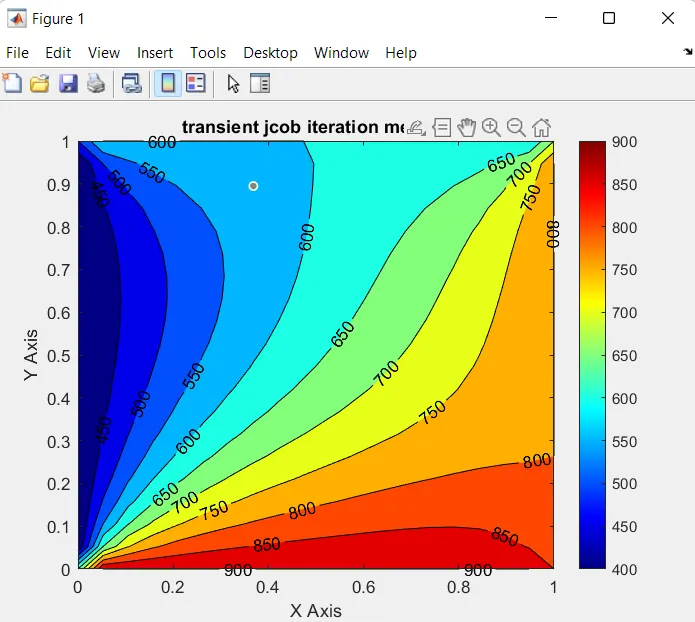
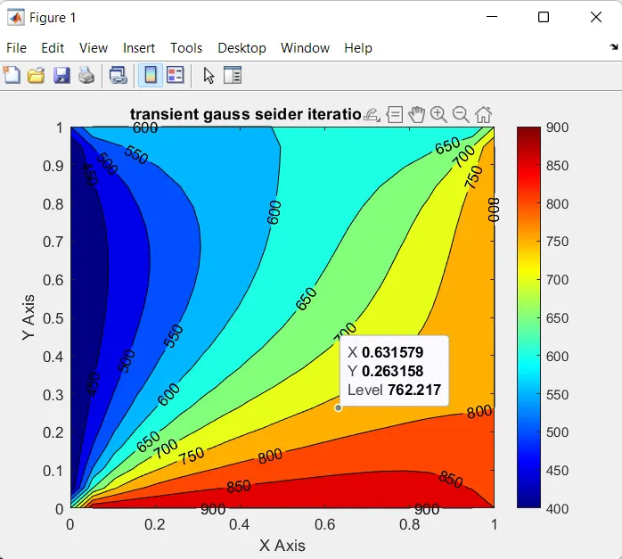
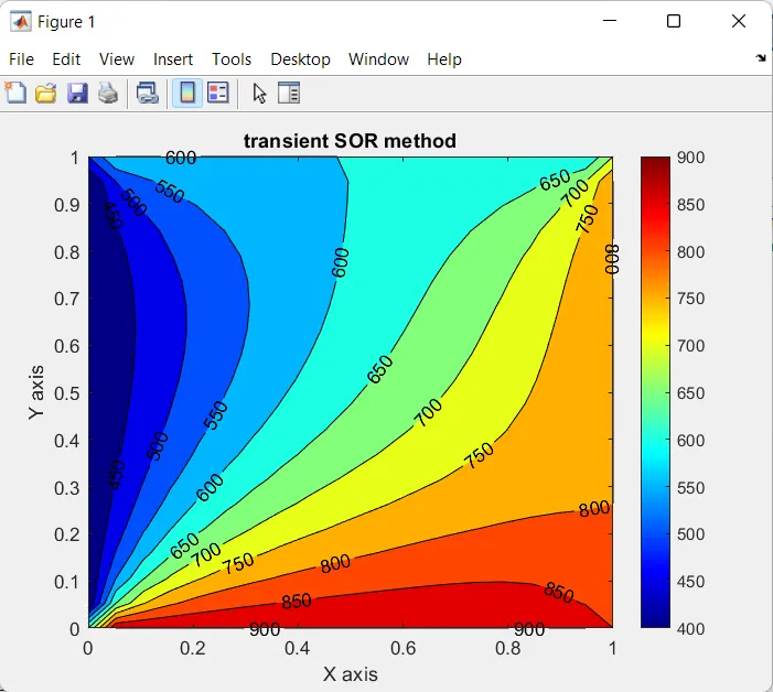
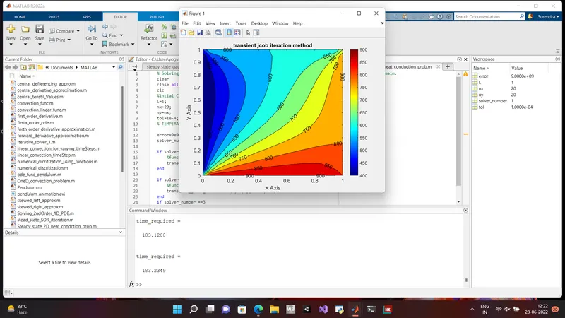
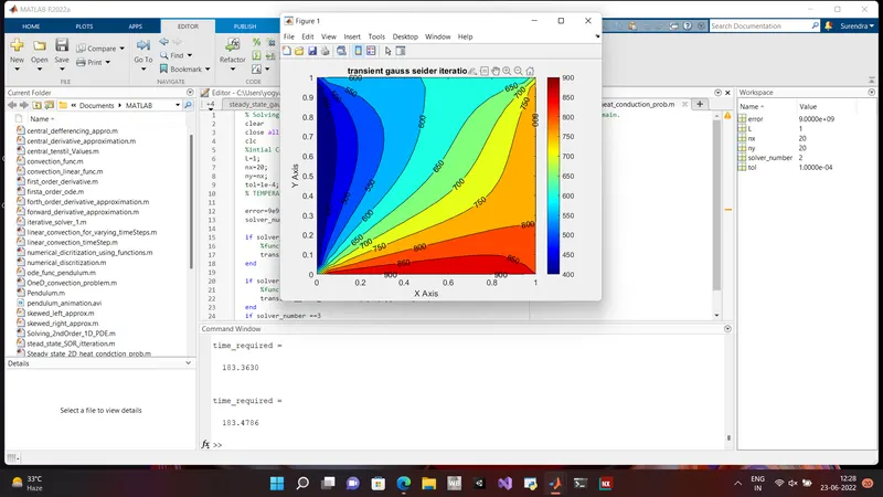
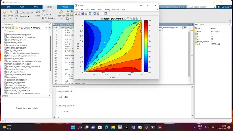
From the above plots you can conclude that explicit method takes less time to execute but when it comes to stability it mainly depend on CFL condition if this condition is not satisfied the solution gets blow up.Where as in the implicit methods jacobian method gives the solution in 7970 iterations where as gauss method takes 6629 iterations but using SOR method you get the solution in 5098 iterations but the computational tine high for SOR and then jacobian but for the gauss method is is faster than other two.Here in SOR method if you use omega value more or less than 1.06 you can see the iteration count increases when it crosses 1.9 then you see that the solution got blew up.so its value should be given less than 2.you can also observe that for any values of alpha dx and dt the solution will be stable, like explicit it is not dependent of CFL condition.