Week 5.1 - Mid term project - Solving the steady and unsteady 2D heat conduction problem
The following observations were made :
- If the alpha values is less then the temperature distribution at the end of time does not reach steady state
- higher values of omega are actually taking more iterations than Gauss-Seidal method. So, a relatively low value (omega=1.1) was taken in this case
- If delta t is low value then it takes more iterations to solve the problem
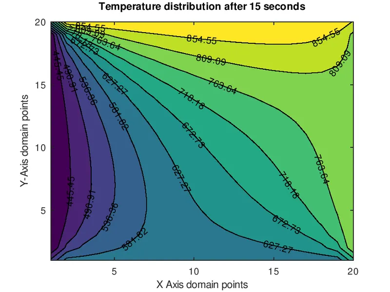

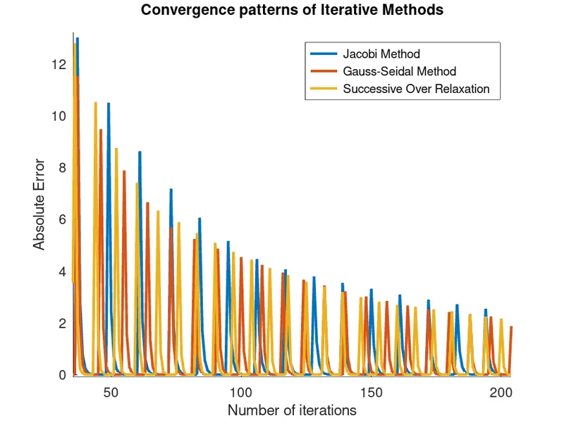
% Solve the steady 2D heat conduction equation % d = partial derivative % dT/dt = alpha (d^2T / dx^2 + d^2T / dy^2) % Boundary Conditions % T_top = 600 K % T_bottom = 900 K % T_left = 400 K % T_right = 800 K clear all; clc; % Parameters nx = 20; % Number of points ny = nx; % Assuming Square domain delta_x = 1; % Stepping in X direction delta_y = 1; % Stepping in Y direction delta_t = 0.1; % Time stepping x = linspace(0,1, nx); % Domain y = linspace(0,1, ny); % Domain tol = 1e-4; % Tolerance to decide if the solution has converged or not T_top = 600; T_bottom = 900; T_left = 400; T_right = 800; alpha = 1.5; % Thermal diffusitivity omega = 1.1; % Relaxation term time = 15; % Total run time of analysis T = 675*ones(nx, ny); % Initializing with average temperature T(:, 1) = T_left; % Boundary Condition T(:, end) = T_right; % Boundary Condition T(1, :) = T_top; % Boundary Condition T(end, :) = T_bottom; % Boundary Condition T(1,1) = (T_top + T_left)/2; % Corner Boundary Condition T(end,1) = (T_bottom + T_left)/2; % Corner Boundary Condition T(1,end) = (T_top + T_right)/2; % Corner Boundary Condition T(end,end) = (T_bottom + T_right)/2; % Corner Boundary Condition hold on; T_init = T; k = 2*(delta_x^2 + delta_y^2)/(delta_x^2 * delta_y^2); %%%%%%%%%% Explicit Method %%%%%%%%%% T_old = T_init; error = tol+0.1; % so that the while loop actually starts for t=1:time/delta_t for i=2:nx-1 for j=2:ny-1 T(i,j) =T_old(i,j) + alpha*delta_t*( (T_old(i+1,j)-2*T_old(i,j)+T_old(i-1,j))/delta_x^2 + T_old(i,j+1)-2*T_old(i,j)+T_old(i,j-1)/delta_y^2 ); end end T_old = T; end T_explicit = T; k1 = alpha*delta_t/delta_x^2; k2 = alpha*delta_t/delta_y^2; term = 1/(1 + 2*k1 + 2*k2); %%%%%%%%%% Jacobi Method %%%%%%%%%% T_old = T_init; T_timeold = T_old; iter = 1; % to keep a record of number of iterations jacobi_error = zeros(2); for t=1:time/delta_t error = tol+0.1; % so that the while loop actually starts while error > tol for i=2:nx-1 for j=2:ny-1 % Central scheme for 2nd order derivative T(i,j) =term*( T_timeold(i,j) +k1*(T_old(i+1,j)+T_old(i-1,j)) +k2*(T_old(i,j+1)+T_old(i,j-1)) ); end end % T-T_old is a (nx X ny) matrix. So, the max value gives the max value of each column. This forms another matrix. We need to take the max of this matrix again to get the max of all values in that matrix error = max(max(abs(T-T_old))); jacobi_error(iter,1) = iter; % storing the iteration value jacobi_error(iter,2) = error; % storing the error value T_old = T; iter = iter + 1; end T_timeold = T; end fprintf('Jacobi Method \n') fprintf('After %d iterations, solution converged with error of %8.7f\n', iter, error) figure(1) plot(jacobi_error(:,1), jacobi_error(:,2), 'LineWidth', 2) %%%%%%%%%% Gauss-Seidal Method %%%%%%%%%% T_old = T_init; T_timeold = T_old; iter = 1; % to keep a record of number of iterations gs_error = zeros(2); for t=1:time/delta_t error = tol+0.1; % so that the while loop actually starts while error > tol for i=2:nx-1 for j=2:ny-1 % Central scheme for 2nd order derivative T(i,j) =term*( T_timeold(i,j) +k1*(T_old(i+1,j)+T(i-1,j)) +k2*(T_old(i,j+1)+T(i,j-1)) ); end end % T-T_old is a (nx X ny) matrix. So, the max value gives the max value of each column. This forms another matrix. We need to take the max of this matrix again to get the max of all values in that matrix error = max(max(abs(T-T_old))); gs_error(iter,1) = iter; % storing the iteration value gs_error(iter,2) = error; % storing the error value T_old = T; iter = iter + 1; end T_timeold = T; end fprintf('Gauss-Seidal Method \n') fprintf('After %d iterations, solution converged with error of %8.7f\n', iter, error) plot(gs_error(:,1), gs_error(:,2), 'LineWidth', 2) %%%%%%%%%% Successive Over Relaxation Method %%%%%%%%%% T_old = T_init; T_timeold = T_old; iter = 1; % to keep a record of number of iterations sor_error = zeros(2); for t=1:time/delta_t error = tol+0.1; % so that the while loop actually starts while error > tol for i=2:nx-1 for j=2:ny-1 % Central scheme for 2nd order derivative T(i,j) =(1-omega)*T_old(i,j) + omega*term*( T_timeold(i,j) +k1*(T_old(i+1,j)+T(i-1,j)) +k2*(T_old(i,j+1)+T(i,j-1)) ); end end % T-T_old is a (nx X ny) matrix. So, the max value gives the max value of each column. This forms another matrix. We need to take the max of this matrix again to get the max of all values in that matrix error = max(max(abs(T-T_old))); sor_error(iter,1) = iter; % storing the iteration value sor_error(iter,2) = error; % storing the error value T_old = T; iter = iter + 1; end T_timeold = T; end fprintf('Successive Over Relaxation Method \n') fprintf('After %d iterations, solution converged with error of %8.7f\n', iter, error) plot(sor_error(:,1), sor_error(:,2), 'LineWidth', 2) xlabel('Number of iterations') ylabel('Absolute Error') title('Convergence patterns of Iterative Methods') legend('Jacobi Method', 'Gauss-Seidal Method', 'Successive Over Relaxation') % xlim([0 100]) % ylim([0 1]) figure(2) contourf(T, 'showtext', 'on') xlabel('X Axis domain points') ylabel('Y-Axis domain points') title('Temperature distribution after 15 seconds')