Week 5.1 - Mid term project - Solving the steady and unsteady 2D heat conduction problem
Problem Statement 1
Solve the 2D heat conduction equation by using the point iterative techniques that were taught in the class. The Boundary conditions for the problem are as follows;
Top Boundary = 600 K
Bottom Boundary = 900 K
Left Boundary = 400 K
Right Boundary = 800 K
2D heat conduction equation is given by :
`(del^2T)/(delx^2) +(del^2T)/(dely^2)=0`
Matlab Program for Steady State:
%Solving 2D Steady-State State heat conduction equation
clear all
close all
clc


%Inputs given
nx =10;
ny =10;
L =1;


x=linspace(0,L,nx);
y=linspace(0,L,ny);
nx = ny;


dx=L/(nx-1);
dy=L/(ny-1);

% error should be greater than tolerance
error=9e9;
tol=1e-4;


%Defining Boundary Conditions
%Top Boundary = 600 K
%Bottom Boundary = 900 K
%Left Boundary = 400 K
%Right Boundary = 800 K


T_T=600;
T_B=900;
T_L=400;
T_R=800;

%Temperature Matrix

T= 298*ones(nx,ny);
T(1,:)=T_B;
T(end,:)=T_T;
T(:,1)=T_L;
T(:,end)=T_R;
omega = 1.2;
Told = T
jacobi_iter =1;

iterative_solver =1;
%jacobi method

if iterative_solver ==1
jacobi_iterations =1;
while(error >tol)
for i=2:nx-1
for j=2:ny-1
T(i,j) =0.25*(Told(i-1,j) +Told(i+1,j)+Told(i,j-1)+Told(i,j+1));
end
end
error = max(max(abs(Told-T)));
Told = T;
jacobi_iterations = jacobi_iterations+1;


%plotting
figure(1)

contourf(T)
pause(0.03)
xlabel('X axis')
ylabel('T')
title_text = ('Jacobian method')
title(title_text)


end
end
error = 9e9;
tol = 1e-4;

% Gauss siedal method


for iterative_solver =2;
%update values
% length of domain and it is a square
L =1;
%nx,ny no of grid points
nx = 10;
ny = nx;
x =linspace(0,L,nx);
y =linspace(0,L,ny);
dx=L/(nx-1);
dy=L/(ny-1);


% Define boundary conditions
T_L = 400;
T_T = 600;
T_R = 800;
T_B = 900;
T = ones(nx,ny);

%Temperature at boundary
T(:,1)=T_L;
T(:,end)=T_R;
T(end,:)=T_T;
T(1,:)=T_B;
SOR_iterations =1;


if iterative_solver ==2
SOR_iterations =1;
while(error >tol)
for i=2:nx-1
for j=2:ny-1
T(i,j) =0.25*(T(i-1,j) +Told(i+1,j)+T(i,j-1)+Told(i,j+1));
end
end
error = max(max(abs(Told-T)));
Told = T;
SOR_iterations = SOR_iterations+1;
end
end

%plotting
figure(2)

contourf(T)
pause(0.03)
xlabel('X axis')
ylabel('T')
title_text = ('Gauss Siedel method')
title(title_text)
end


% SOR method


for iterative_solver =3;
%update values
% length of domain and it is a square
L =1;
%nx,ny no of grid points
nx = 10;
ny = nx;
x =linspace(0,L,nx);
y =linspace(0,L,ny);
dx=L/(nx-1);
dy=L/(ny-1);
error = 9e9;
tol = 1e-4;

% Define boundary conditions
T_L = 400;
T_T = 600;
T_R = 800;
T_B = 900;
T = 298*ones(nx,ny);

%Temperature at boundary
T(:,1)=T_L;
T(:,end)=T_R;
T(end,:)=T_T;
T(1,:)=T_B;
SOR_iterations =1;


if iterative_solver ==3
SOR_iterations =1;
while(error >tol)
for i=2:nx-1
for j=2:ny-1
T(i,j) =((1-omega)*Told(i,j)+(omega*0.25*(T(i-1,j)+Told(i+1,j)+T(i,j-1)+Told(i,j+1))));
end
end
error = max(max(abs(Told-T)));
Told = T;
SOR_iterations = SOR_iterations+1;
end
end

%plotting
figure(3)

contourf(T)
pause(0.03)
title_text = ('SOR method')
title(title_text)
xlabel('X axis')
ylabel('T')
end
Output :
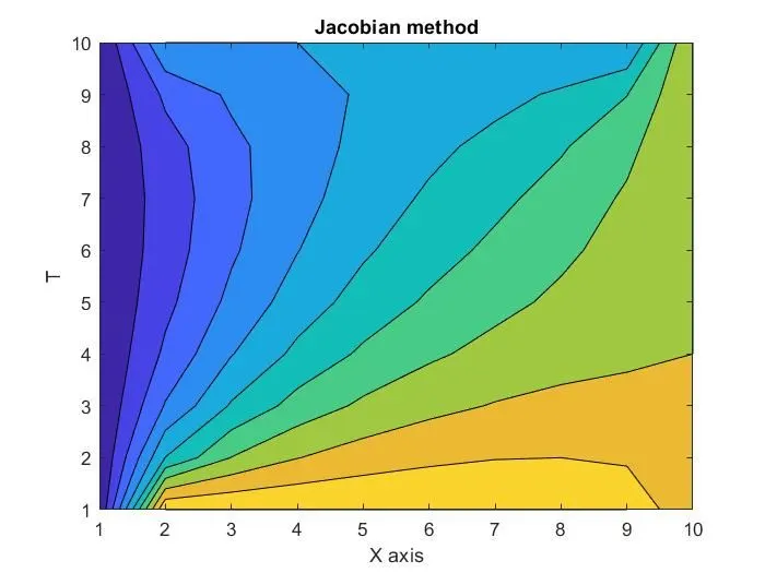
1) Jacobian method :
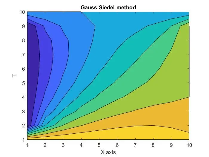
2) Gauss Siedel method :
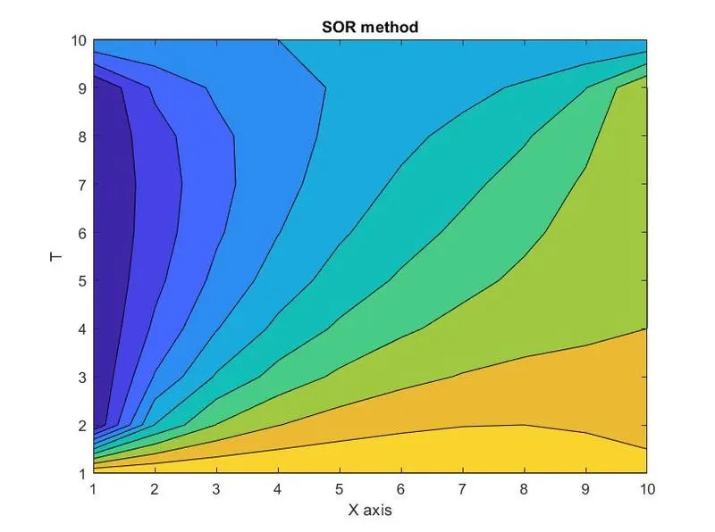
3) SOR Method :
Unsteady state heat conduction equation in 2D is given by :
`(delT)/(delt) = alpha*((del^2T)/(delx^2) + (del^2T)/(dely^2))`
By rearranging the above equation, we get the following equation :
`T_p^(n+1) =T_p^n +K_1*(T_L-2*T_P+T_R)^n+K_2*(T_T-2*T_P+T_B)^n`
where `K_1 = (alpha*Deltat)/(Deltax^2)`
`K_2 = (alpha*Deltat)/(Deltay^2)`
1) Implicit Method :
`T_P^(n+1)= (term1)*T_P^(n) +(term2)*(T_L+T_R)^(n+1)+(term3)*(T_T+T_B)^(n+1)`
where
`K_1 = (alpha*Deltat)/(Deltax^2)`
`K_2 = (alpha*Deltat)/(Deltay^2)`
where term 2 = K1*term1
term3 = K2*term1
`term1 = 1/(1+2*K1+2*K2)`
Matlab program :
clear all;
close all;
clc;


%inputs
L =1;
nx = 25
ny = nx;
x =linspace(0,L,nx);
y =linspace(0,L,ny);
dx = x(2)-x(1);
dy = y(2)-y(1);
error = 9e9;
tol = 1e-4;
dt=0.1;
alpha = 1.4;
t=10;

%CFL number
N = alpha*dt/(dx^2);

% Define boundary conditions
T_L = 400;
T_T = 600;
T_R = 800;
T_B = 900;
T = 298*ones(nx,ny);
T(:,1)=T_L;
T(:,end)=T_R;
T(end,:)=T_B;
T(1,:)=T_T;


% Average Temperature at corner
T(1,1) = (T_T+T_L)/2;
T(1,end) = (T_T+T_R)/2;
T(end,1) = (T_L+T_B)/2;
T(end,end) = (T_R+T_B)/2;


%Calculation

k1 = (alpha*dt)/(dx^2);
k2 = (alpha*dt)/(dy^2);
nt=t/dt;

%creating a copy of T

Told =T;
T_prev=Told;

%jacobi method

nt= t/dt;
iterative_solver =1;
jacobi_iterations =1;
for g=1:nt
if iterative_solver ==1
term1=(1+2*k1+2*k2)^(-1);
term2=k1*term1;
term3=k2*term2;


while(error >tol)
for i=2:nx-1
for j=2:ny-1
H=(Told(i-1,j)+Told(i+1,j));
V=(Told(i,j-1)+Told(i,j+1));
T(i,j)=(T_prev(i,j)*term1)+(H*term2)+(V*term3);

end
end
error = max(abs(Told-T));
Told = T;
jacobi_iterations = jacobi_iterations+1;
end
T_prev=T;
end

%Plotting
figure(1)
contour(T)
title_text = ('Jacobi Method')
title(title_text)

xlabel('Xaxis');
ylabel('Yaxis');
pause(0.03);
end

%Gauss seidel method
%inputs
L =1;
nx = 25;
ny = nx;
x =linspace(0,L,nx);
y =linspace(0,L,ny);
dx = x(2)-x(1);
dy = y(2)-y(1);
error = 9e9;
tol = 1e-4;
dt=0.1;
t=10;
alpha = 1.4;

%CFL number

N= alpha*dt/(dx^2);
% Define boundary conditions
T_L = 400;
T_T = 600;
T_R = 800;
T_B = 900;
T = 298*ones(nx,ny);
T(:,1)=T_L;
T(:,end)=T_R;
T(end,:)=T_B;
T(1,:)=T_T;

% Average Temperature at corner
T(1,1) = (T_T+T_L)/2;
T(1,end) = (T_T+T_R)/2;
T(end,1) = (T_L+T_B)/2;
T(end,end) = (T_R+T_B)/2;

%Calculation
k1 = (alpha*dt)/(dx^2);
k2 = (alpha*dt)/(dy^2);
nt=t/dt;

Told =T;
T_prev=Told;
iterative_solver =2;
gs_iterations =1;
for h = 1:nt
if iterative_solver ==2
term1=(1+2*k1+2*k2)^(-1);
term2=k1*term1;
term3=k2*term2;


while(error >tol)
for i=2:nx-1
for j=2:ny-1
H=(Told(i-1,j)+Told(i+1,j));
V=(Told(i,j-1)+Told(i,j+1));
T(i,j)=(T_prev(i,j)*term1)+(H*term2)+(V*term3);
end
end
error = max(abs(Told-T));
Told = T;

gs_iterations = gs_iterations+1;
end
T_prev=T;
end

%plotting
figure(2)
contourf(T)
title_text=('Gauss Siedel method')
title(title_text);
xlabel('Xaxis');
ylabel('Yaxis');
pause(0.03);
end

%SOR method
%inputs
L =1;
nx = 25;
ny = nx;
x =linspace(0,L,nx);
y =linspace(0,L,ny);
dx = x(2)-x(1);
dy = y(2)-y(1);
error = 9e9;
tol = 1e-4;
dt=0.1;
t=10;
alpha = 1.4;

%CFL number

N= alpha*dt/(dx^2);
% Define boundary conditions
T_L = 400;
T_T = 600;
T_R = 800;
T_B = 900;
T = 298*ones(nx,ny);
T(:,1)=T_L;
T(:,end)=T_R;
T(end,:)=T_B;
T(1,:)=T_T;

% Average Temperature at corner
T(1,1) = (T_T+T_L)/2;
T(1,end) = (T_T+T_R)/2;
T(end,1) = (T_L+T_B)/2;
T(end,end) = (T_R+T_B)/2;

%Calculation
k1 = (alpha*dt)/(dx^2);
k2 = (alpha*dt)/(dy^2);
nt=t/dt;

Told =T;
T_prev=Told;
iterative_solver =2;
SOR_iterations =1;
for h = 1:nt
if iterative_solver ==3
term1=(1+2*k1+2*k2)^(-1);
term2=k1*term1;
term3=k2*term2;


while(error >tol)
for i=2:nx-1
for j=2:ny-1
H=(Told(i-1,j)+Told(i+1,j));
V=(Told(i,j-1)+Told(i,j+1));
T(i,j)=(T_prev(i,j)*term1)+(H*term2)+(V*term3);
end
end
error = max(abs(Told-T));
Told = T;

SOR_iterations = SOR_iterations+1;
end
T_prev=T;
end

%plotting
figure(3)
contourf(T)
title_text=('SOR method')
title(title_text);
xlabel('Xaxis');
ylabel('Yaxis');
pause(0.03);
end
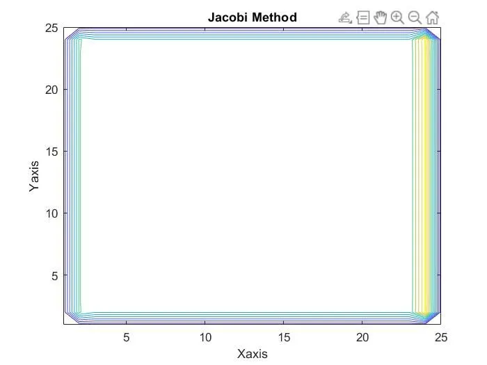
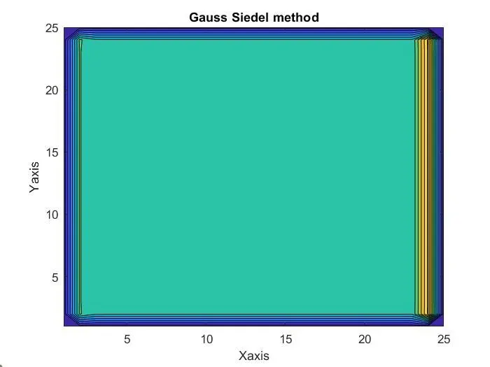
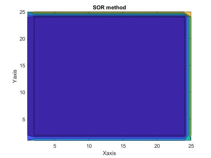
Output :
Explicit Method :
`T_p^(n+1) =T_p^n +K_1*(T_L-2*T_P+T_R)^n+K_2*(T_T-2*T_P+T_B)^n`
where `K_1 = (alpha*Deltat)/(Deltax^2)`
`K_2 = (alpha*Deltat)/(Deltay^2)`
MATLAB Program:
clear all;
close all;
clc;


%inputs
L =1;
nx = 40;
ny = nx;
x =linspace(0,L,nx);
y =linspace(0,L,ny);
dx = x(2)-x(1);
dy = y(2)-y(1);
error = 9e9;
tol = 1e-4;
dt=0.1;
alpha = 1.4;
t=1;
%CFL number
N= alpha*dt/(dx^2);

% Define boundary conditions
T_L = 400;
T_T = 600;
T_R = 800;
T_B = 900;
T = 298*ones(nx,ny);

%Temperature at boundary
T(:,1)=T_L;
T(:,end)=T_R;
T(end,:)=T_B;
T(1,:)=T_T;

% Average Temperature at corner
T(1,1) = (T_T+T_L)/2;
T(1,end) = (T_T+T_R)/2;
T(end,1) = (T_L+T_B)/2;
T(end,end) = (T_R+T_B)/2;

%Calculation

k1 = (alpha*dt)/(dx^2);
k2 = (alpha*dt)/(dy^2);
Told =T;
nt=t/dt;

iterative_solver =1;

iteration =1;
for g =1:nt
if iterative_solver ==1

while(error >tol)
for i=2:nx-1
for j=2:ny-1
term1= Told(i,j);
term2=k1*(Told(i+1,j)-2*Told(i,j)+Told(i-1,j));
term3=k2*(Told(i,j+1)-2*Told(i,j)+Told(i,j-1));
T(i,j)=term1+term2+term3;
end
end
error = max(abs(Told-T));
Told = T;
iteration = iteration+1;
end
end

%plotting
figure(1);
contourf(T);
title_text=('Explicit method')
title(title_text);
xlabel('Xaxis');
ylabel('Yaxis');
pause(0.03);
end
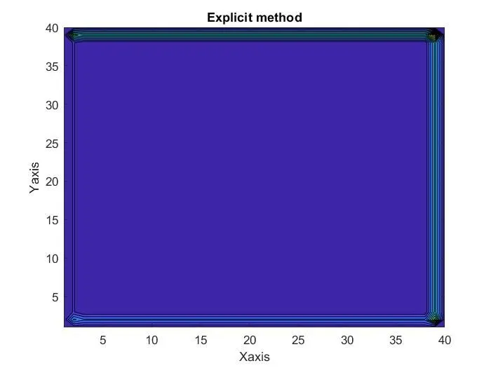
Output :
Conclusion :
from the above, it is concluded that among all three methods i.e. Jacobi, Gauss Siedel, and SOR, SOR method is the most efficient method as it converges faster than other methods with less number of iterations.
Implicit method in the transient state takes more time to converge as compared to the explicit method, But the explicit method can only be used if CFL number is greater than or equal to 0.5 because if the CFL number will be greater than 0.5 then the solution will become unstable.