Week 5.1 - Mid term project - Solving the steady and unsteady 2D heat conduction problem
Steady state analysis & Transient State Analysis
Solve the 2D heat conduction equation by using the point iterative techniques that were taught in the class. The Boundary conditions for the problem are as follows;
Top Boundary = 600 K
Bottom Boundary = 900 K
Left Boundary = 400 K
Right Boundary = 800 K
Heat equation is a partial differential equation the solution of which gives the distribution of temperature in a region as a function of space and time when the temperature at the boundaries, the initial distribution of temperature, and the physical properties of the medium are specified.
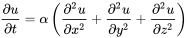
- x,y, and z are the coordinates and t represents the time.
- alpha is the thermal diffusivity of the medium
Steady-state:
When the system reaches an equilibrium state and there is no heat transfer we call it a steady state.
Since it is in equilibrium we don't need to consider the time when we solve the equation.
so the above equation will d^2*u/ dx^2 + d^2*u/ dy^2 =0. As a result, two loops are enough to solve this equation.
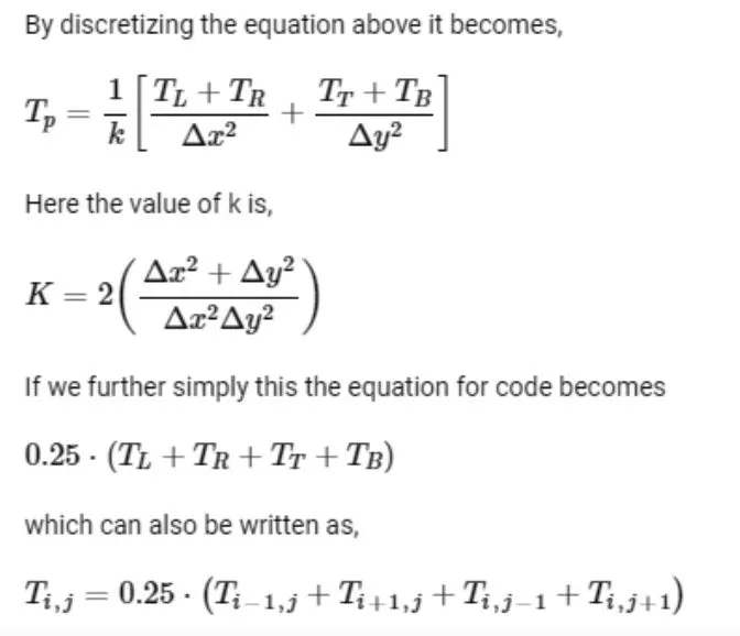
NB: All three solvers for the steady-state equation is in the below program
% Steady state 2d heat conduction equation
close all
clear all
clc
% grid points and boundary conditions
nx=10;
ny=nx;

x= linspace(0,1,nx);
y= linspace(0,1,ny);

dx= x(2)-x(1);
dy= y(2)-y(1);

%T matrix

T= 300* ones(nx,ny);
% initial condition
T(2:ny-1,1)= 400;
T(1, 2:nx-1)=600;
T(2:ny-1,nx)= 800;
T(ny, 2:nx-1)=900;

%  temp at corner points
T(1,1) = (400+600)/2;
T(1,ny) = (800+600)/2;
T(nx,1)=(900+400)/2 ;
T(nx,ny)=(900+800)/2;


Told=T;
% solver 1: Jacobi
% solver 2: Gauss-Siedel
% Solver 3: Successive over relaxation

%select the solver below
solver=3;
% Solving the equation by Jacobi method


error = 1;

tol = 1e-4;

if solver==1
    iter=1;

    while(error > tol)
        for i = 2:nx-1
            for j= 2:ny-1
                T(i,j)= 0.25*(Told(i-1,j) + Told(i+1,j) + Told(i,j-1) + Told(i,j+1));
            end
        end

        error = max(max(abs(Told-T)));

        Told = T;
        iter = iter + 1;
    end
end

% Solving the equation by Gauss-Siedel


if solver==2
    iter=1;

    while(error > tol)
        for i = 2:nx-1
            for j= 2:ny-1
                T(i,j)= 0.25*(T(i-1,j) + Told(i+1,j) + T(i,j-1) + Told(i,j+1));
            end
        end

        error = max(max(abs(Told-T)));

        Told = T;
        iter = iter + 1;
    end
end
% Successive over relaxation

if solver==3
    iter=1;
    omega=1.2;
    while(error > tol)
        for i = 2:nx-1
            for j= 2:ny-1
                T(i,j)= omega*( 0.25*(T(i-1,j) + Told(i+1,j) + T(i,j-1)+ Told(i,j+1))) +(1-omega)* Told(i,j);
            end
        end

        error = max(max(abs(Told-T)));

        Told = T;
        iter = iter + 1;
    end
end


% plotiing

figure(1)
T=flip(T);
contourf (T)
clabel (contourf(T))
colorbar
colormap(jet)
%set(gca,'ydir','reverse')

xlabel('X-Axis')
ylabel('Y-axis')

title(sprintf( 'No. of iterations= %d' ,iter))

pause(0.03);
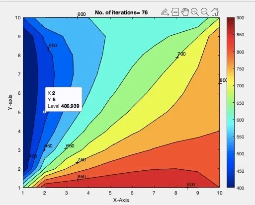
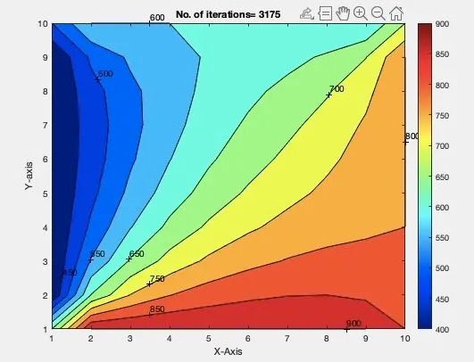
Jacobi method
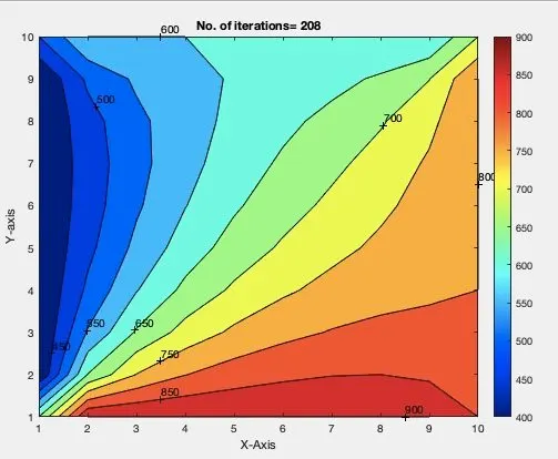
Gauss-Seidel method
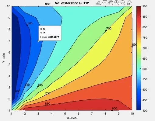
Successive over relaxation method
_____________________________________________________________________________________________________________________________________________________________________________________________________________________________________________________________________________________________
Unsteady state:
This is the state before the equilibrium, where the time maters. When we solve the unsteady equation we need to consider the time. So there will be three loops to solve this equation
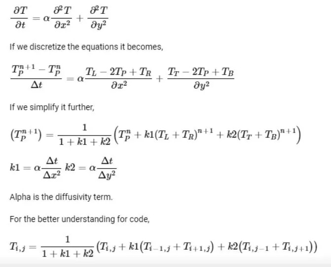
Unsteady state 2d heat conduction equation Jacobi method
% UnSteady state 2d heat conduction equation Jacobi method
close all
clear all
clc
% grid points and boundary conditions
nx=10;
ny=nx;
nt= 1400;
x= linspace(0,1,nx);
y= linspace(0,1,ny);

dx= x(2)-x(1);
dy= y(2)-y(1);

dt = 1e-3;

%T matrix

T= 300* ones(nx,ny);
% initial condition
T(2:ny-1,1)= 400;
T(1, 2:nx-1)=600;
T(2:ny-1,nx)= 800;
T(ny, 2:nx-1)=900;

%  temp at corner points
T(1,1) = (400+600)/2;
T(1,ny) = (800+600)/2;
T(nx,1)=(900+400)/2 ;
T(nx,ny)=(900+800)/2;


Told=T;
Tinitial=T;

% Solving the equation by Jacobi method

% defining constant
k1= 1.1*(dt/(dx^2));
k2= 1.1*(dt/(dy^2));


error = 1;

tol = 1e-4;
iteration_no =1;


for k =1:nt
    error = 5
    while (error > tol)
        for i =2:nx-1
            for j = 2:ny-1

                A = 1/( 1+ (2*k1) + (2*k2));
                B = k1*A;
                C = k2*A;
                D = (Told(i-1,j))+ (Told(i+1,j));
                E = (Told(i,j-1))+ (Told(i,j+1));

                T(i,j) = ( Tinitial(i,j)* A) + (D*B) + (E*C);
            end
        end
        error = max(max(abs(Told -T)));
        Told = T;
        iteration_no = iteration_no + 1;
    end

    Tinitial=T;


end


figure(1)
    T=flip(T);
    contourf (T)

    clabel (contourf(T))
    colorbar
    colormap(jet)
    %set(gca,'ydir','reverse')

    xlabel('X-Axis')
    ylabel('Y-axis')

    title(sprintf( 'No. of iterations= %d' ,iteration_no))

    pause(0.03);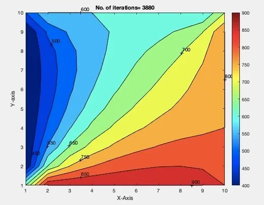
Gauss-Siedel method implicit
% UnSteady state 2d heat conduction equation Gauss-Siedel
close all
clear all
clc
% grid points and boundary conditions
nx=10;
ny=nx;
nt= 1400;
x= linspace(0,1,nx);
y= linspace(0,1,ny);

dx= x(2)-x(1);
dy= y(2)-y(1);

dt = 1e-3;

%T matrix

T= 300* ones(nx,ny);
% initial condition
T(2:ny-1,1)= 400;
T(1, 2:nx-1)=600;
T(2:ny-1,nx)= 800;
T(ny, 2:nx-1)=900;

%  temp at corner points
T(1,1) = (400+600)/2;
T(1,ny) = (800+600)/2;
T(nx,1)=(900+400)/2 ;
T(nx,ny)=(900+800)/2;


Told=T;
Tinitial=T;

% Solving the equation by Jacobi method

% defining constant
k1= 1.1*(dt/(dx^2));
k2= 1.1*(dt/(dy^2));


error = 1;

tol = 1e-4;
iteration_no =1;


for k =1:nt
    error = 5;
    while (error > tol)
        for i =2:nx-1
            for j = 2:ny-1

                A = 1/( 1+ (2*k1) + (2*k2));
                B = k1*A;
                C = k2*A;
                D = (T(i-1,j))+ (T(i+1,j));
                E = (T(i,j-1))+ (T(i,j+1));

                T(i,j) = ( Tinitial(i,j)* A) + (D*B) + (E*C);
            end
        end
        error = max(max(abs(Told -T)));
        Told = T;
        iteration_no = iteration_no + 1;
    end

    Tinitial=T;


end

figure(1)
    T=flip(T);
    contourf (T)

    clabel (contourf(T))
    colorbar
    colormap(jet)
    %set(gca,'ydir','reverse')

    xlabel('X-Axis')
    ylabel('Y-axis')

    title(sprintf( 'No. of iterations= %d' ,iteration_no))

pause(0.03); 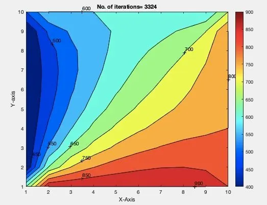
Successive over relaxation
% UnSteady state 2d heat conduction equation Successive over relaxation
close all
clear all
clc
% grid points and boundary conditions
nx=10;
ny=nx;
nt= 1400;
x= linspace(0,1,nx);
y= linspace(0,1,ny);

dx= x(2)-x(1);
dy= y(2)-y(1);

dt = 1e-3;
omega = 1.1;
%T matrix

T= 300* ones(nx,ny);
% initial condition
T(2:ny-1,1)= 400;
T(1, 2:nx-1)=600;
T(2:ny-1,nx)= 800;
T(ny, 2:nx-1)=900;

%  temp at corner points
T(1,1) = (400+600)/2;
T(1,ny) = (800+600)/2;
T(nx,1)=(900+400)/2 ;
T(nx,ny)=(900+800)/2;


Told=T;
Tinitial=T;
Tend= T;

% Solving the equation by Successive over relaxation

% defining constant
k1= 1.1*(dt/(dx^2));
k2= 1.1*(dt/(dy^2));


solver=1;
error = 1;

tol = 1e-4;
iteration_no =1;


for k =1:nt
    error = 5;
    while (error > tol)
        for i =2:nx-1
            for j = 2:ny-1

                A = 1/( 1+ (2*k1) + (2*k2));
                B = k1*A;
                C = k2*A;
                D = (T(i-1,j))+ (T(i+1,j));
                E = (T(i,j-1))+ (T(i,j+1));

                T(i,j) = ( Tinitial(i,j)* A) + (D*B) + (E*C);
                Tend(i,j) = ((1-omega)* Told(i,j)) + (T(i,j)*omega);
            end
        end
        error = max(max(abs(Told -T)));
        Told = Tend;
        iteration_no = iteration_no + 1;
    end

    Tinitial=Tend;


end


figure(1)
    T=flip(T);
    contourf (T)

    clabel (contourf(T))
    colorbar
    colormap(jet)
    %set(gca,'ydir','reverse')

    xlabel('X-Axis')
    ylabel('Y-axis')

    title(sprintf( 'No. of iterations= %d' ,iteration_no))

    pause(0.03);
Unsteady Explicit solution
% UnSteady state 2d heat conduction equation
close all
clear all
clc
% grid points and boundary conditions
nx=10;
ny=nx;
nt= 1400;
x= linspace(0,1,nx);
y= linspace(0,1,ny);

dx= x(2)-x(1);
dy= y(2)-y(1);

dt = 1e-3;
omega = 1.1;
%T matrix

T= 300* ones(nx,ny);
% initial condition
T(2:ny-1,1)= 400;
T(1, 2:nx-1)=600;
T(2:ny-1,nx)= 800;
T(ny, 2:nx-1)=900;

%  temp at corner points
T(1,1) = (400+600)/2;
T(1,ny) = (800+600)/2;
T(nx,1)=(900+400)/2 ;
T(nx,ny)=(900+800)/2;


Told=T;
Tinitial=T;
Tend= T;

% Solving the equation by Explicit

% defining constant
k1= 1.1*(dt/(dx^2));
k2= 1.1*(dt/(dy^2));


solver=1;
error = 1;

tol = 1e-4;
iteration_no =1;

error = 5;
for k =1:nt

    while (error > tol)
        for i =2:nx-1
            for j = 2:ny-1

                A = Told(i,j);
                B = k1*(Told(i+1,j)-2*Told(i,j)+(Told(i-1,j)));
                C = k2*(Told(i,j+1)-2*Told(i,j) + Told(i,j-1));
                T(i,j) = A+B+C;


            end
        end
        error = max(max(abs(Told -T)));
        Told = T;
        iteration_no = iteration_no + 1;
    end


end

  figure(1)

    contourf (T)

    clabel (contourf(T))
    colorbar
    colormap(jet)
    set(gca,'ydir','reverse')

    xlabel('X-Axis')
    ylabel('Y-axis')

    title(sprintf( 'No. of iterations= %d' ,iteration_no))

    pause(0.03);
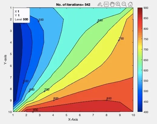
It is obvious from the results that Successive over-relaxation method is most efficient since it required less number of iteration compared to the Jacobi and Gauss-Siedel.
Jacobi is the least efficient method since it is taking more iteration than the other two.
The steady analysis takes less time and iteration since it doesn’t have a time loop.